# ⚡ Type this in your document
data("mtcars")Chapter 10: And, Or, and Membership
Logical operators for filtering data frames
Overview
In Chapter 8, you learned how bracket subsetting works: df[rows, cols] lets you extract and modify exactly the pieces of a data frame you need. This chapter strengthens that skill by adding three essential logical operators to your toolkit: & (AND), | (OR), and %in% (in set). Most real analysis questions require more than one condition: “keep rows where X is true and Y is true,” “keep rows where A or B is true,” or “keep rows where a value is one of several allowed options.”
You will practice translating those English rules into correct R code using logical tests (>, <, ==, !=) combined with &, |, and %in%. You will also practice checking your first interpretation instead of assuming that code is correct just because it ran. That is the open-mindedness focus for this chapter: write the filter you think matches the question, verify the result, and stay willing to revise the code when the output does not match the sentence you meant to write.
By the end of Chapter 10, you will be able to:
✂️ Apply bracket subsetting
x[i, j]to select or exclude rows and columns by position.⚖️ Generate and interpret logical vectors using relational operators (
>,<,<=,>=,==,!=) on data-frame columns accessed with$.🔍 Use logical vectors inside
[ ]to filter rows based on conditions.🔄 Explain and use logical negation with
!to invert tests.🧺 Combine multiple filtering conditions using
&(AND),|(OR), and%in%(membership) to construct multi-criteria subsets.🩹 Diagnose and correct a precedence bug by adding grouping parentheses.
🚜 Construct readable, reproducible multi-condition filters with clear comments and verification checks.
🤔 Compare more than one valid filtering approach and choose the one that is easier to read, check, and explain.
Keep these goals in mind as you move through each section.
Activity Setup
This chapter models an R Notebook, which keeps code, output, and memo notes together. If you have already learned to use Quarto, you may work in a .qmd file instead. Chapter 11 will introduce Quarto to everyone. As you work, notice how your document helps you run code, inspect output, and explain your choices.
Create and Save Your Chapter 10 Document
🎯 Create an R Notebook for the guided activity, or use a Quarto document if you already know how. Save it in your work folder. The example below uses Intro_to_R/Module_5/; follow your instructor’s folder directions if they differ.
Open an R Notebook: Go to
File > New File > R Notebook.Edit the YAML header so it looks like this:
---
title: "Chapter 10 Notes: And, Or, and Membership"
author: "[Your Name]"
date: "`r Sys.Date()`"
output: html_notebook
---
Change
[Your Name]to your actual name. Remove the starter text in the document body below the YAML header, but keep the header and both---lines.Save your R Notebook:
File>Save As..., choose your work folder, and name the filechapter10_notes.Rmd.
Example file structure:
Intro_to_R/
└── Module_5/
    └── chapter10_notes.Rmd
✅ Check that your file name ends in .Rmd and that it is saved in the folder you chose.
NoteAlready using Quarto?
You may create a Quarto document through File > New File > Quarto Document and save it in the same work folder as chapter10_notes.qmd. Use this YAML header:
---
title: "Chapter 10 Notes: And, Or, and Membership"
author: "[Your Name]"
date: today
format:
  html:
    embed-resources: true
---
Replace [Your Name]. Keep the YAML header; remove only unwanted starter text below it. Use the same R code and memo prompts in either format. Knit an .Rmd file or Render a .qmd file to make an HTML report.
🗣 Your document will hold your Chapter 10 code, output, and memo notes. Keeping those pieces together makes it easier to rerun your work, check your filters, and explain the logic behind your subsetting choices.
🤔 If you have used both formats, compare how each helps you see code, output, and memos. Which format makes your work easier to check and explain?
🧶 Knit or render to check your document.
Data for This Chapter
This chapter uses the built-in 🚗 mtcars dataset, so you do not need to download or move a data file for this guided activity.
🎯 Load the dataset inside your document.
✅ Check that mtcars appears in your Environment pane.
🗣 The data() function loads a built-in dataset that already comes with R. Because mtcars is built in, this chapter lets you focus on logical filters and subsetting without also managing an external CSV or Excel file.
🧶 Knit or render to check your document.
Basic Data Inspection
After loading data, inspect it before you start subsetting. You need to know what columns are available, what the values look like, and whether the dataset matches your expectations.
🎯 Open the help file and spreadsheet view for mtcars.
Run these two inspection commands in the Console. They open RStudio panes, so they do not need to run when you knit or render your document. Record what you learn in a memo.
# ⚡ Run these in the Console
?mtcars       # opens the help file in the Help tab
View(mtcars)  # opens the spreadsheet view in the top-left pane
✅ Check the Help tab for variable names and descriptions. Check the spreadsheet view to see the rows and columns.
🗣 The help file gives you information about the dataset, including variable descriptions and source information. The spreadsheet view lets you inspect the data visually before writing subsetting code.
🤔 The column name wt might make you think its values are in pounds. Check the help file before using a weight cutoff: it defines wt in thousands of pounds. Let that description change how you interpret a condition such as wt < 3.
📖 Review: Subsetting template
📜 The SYNTAX: x[i, j]
iis the row index.jis the column index.- Leave
ROWSblank → keep all rows. - Leave
COLUMNSblank → keep all columns.
🎯 Use bracket subsetting to preview the first 6 rows of mtcars.
# ⚡ Type this in your document
mtcars[1:6, ]
mpg cyl disp hp drat wt qsec vs am gear carb
Mazda RX4 21.0 6 160 110 3.90 2.620 16.46 0 1 4 4
Mazda RX4 Wag 21.0 6 160 110 3.90 2.875 17.02 0 1 4 4
Datsun 710 22.8 4 108 93 3.85 2.320 18.61 1 1 4 1
Hornet 4 Drive 21.4 6 258 110 3.08 3.215 19.44 1 0 3 1
Hornet Sportabout 18.7 8 360 175 3.15 3.440 17.02 0 0 3 2
Valiant 18.1 6 225 105 2.76 3.460 20.22 1 0 3 1✅ Check that the output shows the first 6 rows and all columns.
🗣 The blank after the comma means “keep all columns.” This code returns rows 1 through 6 of mtcars with every column included. This gives you a quick preview of the dataset before you start filtering it.
🤔 This preview shows only six rows. It can help you understand the columns, but it cannot show every value in the dataset. Keep that limit in mind when you make claims about what a later filter should return.
🧶 Knit or render to check your document.
Now that you have loaded and inspected mtcars, you are ready to subset it. The next section starts with one way to exclude rows or columns by position, then moves into logical tests that filter rows based on the values inside the data.
Exclude Columns and Rows
Instead of keeping rows/columns by position or condition, you can also drop them. This is often done with negative indices or with logical conditions that create TRUE/FALSE vectors.
Negative Indices
Negative indexing drops rows or columns by position. Inside the bracket subsetting operator [ for vectors/matrices/data frames, a negative integer index means “leave these positions out.”
📜 The SYNTAX: x[-i, -j]
Using negative indices drops rows/columns by position.
🎯 Drop columns 8 and 9 of mtcars to create a new data frame called no_cat. These columns, vs and am, are numeric indicator variables that represent categories.
# ⚡ Type this in your document
no_cat <- mtcars[ , -c(8, 9)]
# ✅ Verify
head(no_cat)
mpg cyl disp hp drat wt qsec gear carb
Mazda RX4 21.0 6 160 110 3.90 2.620 16.46 4 4
Mazda RX4 Wag 21.0 6 160 110 3.90 2.875 17.02 4 4
Datsun 710 22.8 4 108 93 3.85 2.320 18.61 4 1
Hornet 4 Drive 21.4 6 258 110 3.08 3.215 19.44 3 1
Hornet Sportabout 18.7 8 360 175 3.15 3.440 17.02 3 2
Valiant 18.1 6 225 105 2.76 3.460 20.22 3 1🗣 The -c(8, 9) is the integer vector containing -8 and -9. Negative column indices mean: drop column 8 and drop column 9. The blank before the comma, i is empty → all rows. For mtcars, columns 8 and 9 are vs and am, respectively. So mtcars[ , -c(8, 9)] returns all rows and all columns except vs and am.
💡 Tip: Within a single row or column index vector, use positive positions to keep or negative positions to drop. Mixing positive and negative positions in that same vector triggers the error “only 0’s may be mixed with negative subscripts.”
🤔 Negative indexing is useful when you know the exact positions you want to drop. Stay open-minded about whether position is the best choice: if the column order changes, position-based code could remove the wrong columns.
The use of the negative sign - is one way to subset by excluding columns. However, the most powerful way to subset data frames is with logical operators that create TRUE/FALSE vectors.
Inequality !=
Conditional subsetting with logical (relational) operators is more flexible than negative indexing because you can specify conditions on the values in the data frame, not just positions. Recall from Chapter 8 that logical tests create TRUE/FALSE vectors used inside of [ ].
Not Equal To (!=) is a relational operator that compares values and returns a logical vector of TRUE/FALSE results. When the element value is not equal to the specified value, the result is TRUE. When the element value is equal to the specified value, the result is FALSE. The result is the opposite of the == operator, which tests for equality.
🎯 Use != to create a logical vector that is TRUE where the number of cylinders (cyl) is NOT equal to 4.
# ⚡ Type this in your document
mtcars$cyl != 4
[1] TRUE TRUE FALSE TRUE TRUE TRUE TRUE FALSE FALSE TRUE TRUE TRUE
[13] TRUE TRUE TRUE TRUE TRUE FALSE FALSE FALSE FALSE TRUE TRUE TRUE
[25] TRUE FALSE FALSE FALSE TRUE TRUE TRUE FALSE🗣 This does not return a subset. It produces a logical vector you can use for subsetting, typically rows. In this example, the code returns a logical vector with TRUE where the number of cylinders is anything but 4 and FALSE otherwise.
🤔 This is a logic-translation moment. “Not equal to 4” and “exclude the 4-cylinder cars” describe the same idea from different angles. Before you subset, ask whether your code matches the sentence you mean.
📖 Review: Accessing Columns with $
$extracts a single column as a vector.📜 The SYNTAX:
dataframe$column_name
🎯 Use $ to access the cyl column of mtcars as a vector.
# 📖 Review
mtcars$cyl
[1] 6 6 4 6 8 6 8 4 4 6 6 8 8 8 8 8 8 4 4 4 4 8 8 8 8 4 4 4 8 6 8 4🗣 The $ operator is used to access ONE specific column in a data frame by name. The column name is cyl and it tells the number of cylinders: 4, 6, or 8 for each car. The vector lists the values in cyl in row order. The TRUE and FALSE vector returned from mtcars$cyl != 4 returned TRUE when the value did not equal 4.
For example, the first value 6 is TRUE because 6 is not equal to 4. The second value 6 is also TRUE because 6 is not equal to 4. The third value 4 is FALSE because 4 is equal to 4.
🎯 Use the logical test != 4 inside [ ] to keep only rows where cyl is NOT equal to 4.
# ⚡ Type this in your document
not4 <- mtcars[mtcars$cyl != 4, ]
# ✅ Verify
head(not4)
mpg cyl disp hp drat wt qsec vs am gear carb
Mazda RX4 21.0 6 160 110 3.90 2.620 16.46 0 1 4 4
Mazda RX4 Wag 21.0 6 160 110 3.90 2.875 17.02 0 1 4 4
Hornet 4 Drive 21.4 6 258 110 3.08 3.215 19.44 1 0 3 1
Hornet Sportabout 18.7 8 360 175 3.15 3.440 17.02 0 0 3 2
Valiant 18.1 6 225 105 2.76 3.460 20.22 1 0 3 1
Duster 360 14.3 8 360 245 3.21 3.570 15.84 0 0 3 4unique(not4$cyl)[1] 6 8🗣 This returns a subset of mtcars with all rows where the number of cylinders is anything but 4 and all columns. When the logical test returned TRUE, the row is selected. When the logical test returned FALSE, the row is removed from the output.
🤔 The first six rows look right, but they do not prove that every selected car has a cylinder count other than 4. Check unique(not4$cyl) too. If it includes 4, reconsider the logical test before moving on.
Not !
The Not operator ! negates a logical value. !TRUE becomes FALSE, and !FALSE becomes TRUE. It can be used to flip the result of a logical test.
🎯 Use ! to create a subset of mtcars that keeps rows where the number of cylinders (cyl) is NOT equal to 4.
# ⚡ Type this in your document
not4_bang <- mtcars[!(mtcars$cyl == 4), ]
head(not4_bang)
mpg cyl disp hp drat wt qsec vs am gear carb
Mazda RX4 21.0 6 160 110 3.90 2.620 16.46 0 1 4 4
Mazda RX4 Wag 21.0 6 160 110 3.90 2.875 17.02 0 1 4 4
Hornet 4 Drive 21.4 6 258 110 3.08 3.215 19.44 1 0 3 1
Hornet Sportabout 18.7 8 360 175 3.15 3.440 17.02 0 0 3 2
Valiant 18.1 6 225 105 2.76 3.460 20.22 1 0 3 1
Duster 360 14.3 8 360 245 3.21 3.570 15.84 0 0 3 4🗣 !(x == 4) and x != 4 mean the same thing! != is a direct “not equal” comparison. ! is more general. It negates a logical test. Here, !(mtcars$cyl == 4) reads as “NOT (cyl equals 4)”, which is equivalent to “cyl not equal to 4”.
🤔 You just wrote the same filter in two ways. When two approaches give the same result, the next question is which one is easier to read, check, and explain.
🎯 Verify that the ! version of the subset matches the != version.
# ✅ Verify it matches the != version
identical(not4_bang, not4)
[1] TRUE✅ Check that the output returns TRUE.
🗣 The two subsets are the same.
In summary, negative indices - exclude rows/columns by position only. The inequality != operator compares values and returns TRUE/FALSE results, which are useful for filtering rows. The Not ! operator negates any logical test. Not is useful for more complex logical tests such as element-by-element or membership logical operators covered later in this chapter.
Practice Relational Operators
Before we dive into complex logical tests, let’s make sure we understand how relational operators work with subsetting. So far in this chapter, we have used the logical operators ==, !=, and !. Let’s practice using relational operators in combination with subsetting.
Example 1
The Less Than or Equal To (<=) operator returns TRUE where the left side is less than or equal to the right side, and FALSE otherwise.
🎯 Answer the question, “How many cars in the dataset have mpg ≤ 15?” Use a logical test to count how many cars have miles per gallon less than or equal to 15.
# ⚡ Type this in your document in a code chunk
sum(mtcars$mpg <= 15)
[1] 6🗣 The less than or equal to logical test <= 15 evaluates each row value in the column mpg in the mtcars dataset (mtcars$mpg). If the car in a row has a value less than or equal to 15, the result is TRUE, otherwise FALSE. In R, TRUE is treated as 1 and FALSE as 0. The function sum() adds all the TRUE values. There are 6 cars in the mtcars dataset with miles per gallon less than or equal to 15.
🤔 This is a good time to translate code back into words. mtcars$mpg <= 15 means “find cars with mpg less than or equal to 15.” If your words and your code do not match, revise before moving on.
Example 2
The Greater Than or Equal To (>=) operator returns TRUE where the left side is greater than or equal to the right side, and FALSE otherwise. We can combine this operator with negative indexing to create a subset of the data frame.
🎯 Create a subset of mtcars that contains rows with hp >= 100, and drops columns 3, 5, and 8:9 by position.
# ⚡ Type this in your document in a code chunk
selection <- mtcars[mtcars$hp >= 100, -c(3, 5, 8:9)]
# ✅ Verify
head(selection)
mpg cyl hp wt qsec gear carb
Mazda RX4 21.0 6 110 2.620 16.46 4 4
Mazda RX4 Wag 21.0 6 110 2.875 17.02 4 4
Hornet 4 Drive 21.4 6 110 3.215 19.44 3 1
Hornet Sportabout 18.7 8 175 3.440 17.02 3 2
Valiant 18.1 6 105 3.460 20.22 3 1
Duster 360 14.3 8 245 3.570 15.84 3 4🗣 mtcars$hp >= 100 keeps only rows where horsepower is at least 100. The -c(3, 5, 8:9) part drops columns 3, 5, 8, and 9 from the result. In other words, it removes those column positions.
💡 Tip: A common mistake is to forget which side the >, < goes to the =. Remember that the = is always on the right side of the operator.
✔️ >=
🚫 =>
🤔 This subset combines two decisions: which rows to keep and which columns to drop. When code does more than one thing, check each part separately in your mind: “What rows am I keeping?” and “What columns am I removing?”
Example 3
We can also verify that we got the expected number of columns in our subset by passing the stored object names through functions. The function ncol() counts columns, and Equal To (==) compares the results.
🎯 Verify that selection has the expected number of columns: 7 columns, since we dropped 4 from the original 11.
# ✅ Verify
ncol(selection) == ncol(mtcars) - length(c(3, 5, 8:9))
[1] TRUE🗣 This checks whether the subset has the expected number of columns after dropping columns 3, 5, 8, and 9.
ncol(selection)counts the number of columns in theselectiondata frame.ncol(mtcars)counts the number of columns in the originalmtcarsdataset, which is 11.length(c(3, 5, 8:9))counts how many columns we dropped, which is 4. Note that we could have written it asc(3, 5, 8, 9).ncol(mtcars)(11) minuslength(c(3, 5, 8:9))(4) gives us the expected number of columns inselection, which is 7.
If it returns TRUE, the subset has the expected number of columns. If it returns FALSE, something went wrong, such as dropping too many or too few columns.
💡 Tip: This check confirms the column count, not the exact column names. If you also want to verify which columns remain, use names(selection).
# ✅ Optional verification
names(selection)
[1] "mpg" "cyl" "hp" "wt" "qsec" "gear" "carb"🤔 A TRUE column-count check tells you that seven columns remain, but the wrong seven columns could still remain. Compare names(selection) with the columns you intended to keep. If they differ, reconsider which positions you dropped.
The next section introduces three new logical operators that help with more complex conditions: & (and), | (or), and %in% (in set).
&, |, %in%
Up to this point, you have used single logical tests inside brackets to pick rows. For example:
mtcars[mtcars$mpg <= 15, ] mpg cyl disp hp drat wt qsec vs am gear carb
Duster 360 14.3 8 360 245 3.21 3.570 15.84 0 0 3 4
Cadillac Fleetwood 10.4 8 472 205 2.93 5.250 17.98 0 0 3 4
Lincoln Continental 10.4 8 460 215 3.00 5.424 17.82 0 0 3 4
Chrysler Imperial 14.7 8 440 230 3.23 5.345 17.42 0 0 3 4
Camaro Z28 13.3 8 350 245 3.73 3.840 15.41 0 0 3 4
Maserati Bora 15.0 8 301 335 3.54 3.570 14.60 0 1 5 8That works when your filter has one requirement.
What if we have multiple requirements?
“I want cars that are automatic AND have
mpg <= 22.”“I want cars with 4 OR 8 cylinders.”
“I want cylinders in the set
{4, 6}.”
This section adds three new logical operators to your R toolkit: And (&), Or (|), and In Set (%in%).
These operators allow us to combine multiple conditions for more complex subsetting.
Here is a summary table showing primary logical operators.
| Operator | Meaning | Example |
|---|---|---|
> |
greater than | mpg > 20 |
< |
less than | mpg < 15 |
== |
equal to | am == 1 |
>= |
greater than or equal to | mpg >= 25 |
<= |
less than or equal to | mpg <= 15 |
! |
not | !(gear %in% c(3, 4)) |
!= |
not equal to | gear != 4 |
& |
and | x > 2 & y == "a" |
| |
or | cyl == 4 | cyl == 8 |
%in% |
in set | region %in% c("West", "South") |
Let’s explore each of these three new operators in more detail. In this section, we’ll build multiple logical tests on columns, combine tests with & and | to form a single condition, and use %in% to match one of many allowed values.
And &
Suppose we have two events: A and B. The and operator & returns TRUE only if both event A and event B are true. It returns FALSE if either event A or event B, or both, are false. The “and” is used to combine two or more conditions where all conditions must be true.
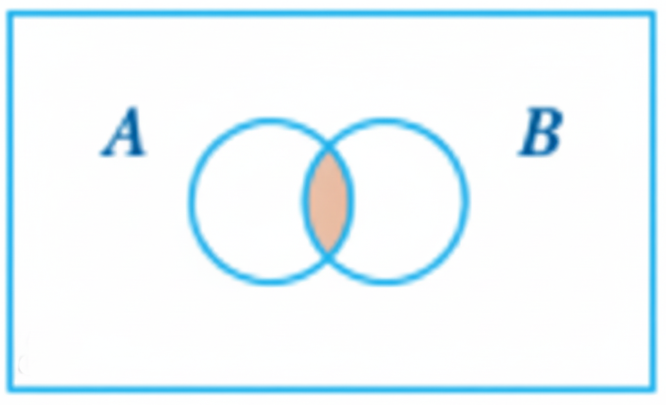
🎯 Filter mtcars to keep cars that are both automatic (am == 0) and have miles per gallon less than or equal to 22.
Step 1: Create two separate logical vectors for each condition.
# ⚡ Type this in your document in a code chunk
is_auto <- mtcars$am == 0
mpg_22_or_less <- mtcars$mpg <= 22

# ✅ Verify: look at the first few TRUE/FALSE values
head(is_auto)
[1] FALSE FALSE FALSE TRUE TRUE TRUEhead(mpg_22_or_less)[1] TRUE TRUE FALSE TRUE TRUE TRUE🗣 Two logical vectors are created. is_auto is TRUE where the car has automatic transmission (am == 0) and FALSE where it has manual transmission (am == 1). mpg_22_or_less is TRUE where the miles per gallon is less than or equal to 22, and FALSE otherwise.
🤔 Creating the conditions separately can make the logic easier to inspect. Before combining them, check whether each individual test means what you think it means.
Step 2: Combine the two logical vectors with & to create a single condition that is TRUE only where both conditions are met.
# ⚡ Combine conditions row-by-row
keep_rows <- is_auto & mpg_22_or_less

# ✅ Verify
head(keep_rows)
[1] FALSE FALSE FALSE TRUE TRUE TRUEsum(keep_rows) # how many rows will be kept?[1] 17🗣 The keep_rows vector is TRUE only where both is_auto and mpg_22_or_less are TRUE. The sum(keep_rows) counts how many rows satisfy both conditions.
🤔 The word and makes the filter stricter. If one condition is TRUE but the other is FALSE, the row is not kept. Check that this matches the data question before you subset.
Step 3: Use the combined logical vector to subset the data frame.
# ⚡ Subset the data
auto_mpg_22_or_less <- mtcars[keep_rows, ]

# ✅ Verify
head(auto_mpg_22_or_less)
mpg cyl disp hp drat wt qsec vs am gear carb
Hornet 4 Drive 21.4 6 258.0 110 3.08 3.215 19.44 1 0 3 1
Hornet Sportabout 18.7 8 360.0 175 3.15 3.440 17.02 0 0 3 2
Valiant 18.1 6 225.0 105 2.76 3.460 20.22 1 0 3 1
Duster 360 14.3 8 360.0 245 3.21 3.570 15.84 0 0 3 4
Merc 280 19.2 6 167.6 123 3.92 3.440 18.30 1 0 4 4
Merc 280C 17.8 6 167.6 123 3.92 3.440 18.90 1 0 4 4🗣 The auto_mpg_22_or_less object is a subset data frame of mtcars that contains only rows where the car is automatic and has miles per gallon less than or equal to 22.
Alternatively, you can combine the conditions directly inside the subset without creating intermediate logical vectors.
# ⚡ Type this in your document in a code chunk
auto_mpg_22_or_less <- mtcars[mtcars$am == 0 & mtcars$mpg <= 22, ]
🗣 Use & when you want rows that satisfy all requirements at the same time. Both mtcars$am == 0 and mtcars$mpg <= 22 must meet the condition to be TRUE.
# ✅ Verify
head(auto_mpg_22_or_less)
# ✅ Verify
nrow(auto_mpg_22_or_less)🗣 & is the correct operator for the creation of auto_mpg_22_or_less because we want cars that are both automatic and have mpg less than or equal to 22. & is strict. It requires everything to be true.
🤔 You have now seen two ways to write the same filter: separate logical vectors first, or one combined condition inside [ ]. When two approaches give the same result, ask which one is easier to read, check, and explain.
💡 Tip: Students often write one condition correctly and “half-write” the other, like this:
mtcars$am == 0 & mpg <= 22That code fails because mpg is a column of mtcars, not a separate object here. Write mtcars$mpg <= 22 for the second condition. You can also combine logical vectors that you created earlier, as you did with is_auto & mpg_22_or_less.
The next section uses |, which answers a different kind of question. Use & when all conditions must be true. Use | when at least one condition can be true.
Or |
Suppose we have two events: A and B. The or logical operator | returns TRUE if either event A is true, event B is true, or both events are true. It only returns FALSE if both events are false. “Or” is inclusive and is used to combine two or more conditions where at least one condition must be true.
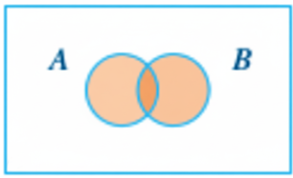
Use | when you want rows that satisfy at least one requirement. The | is located above the Enter key on your keyboard. It is the vertical bar and shares the key with the backslash \. Click and hold the Shift key to type |.
🎯 Keep rows for cars that have either 4 or 8 cylinders.
# ⚡ Type this in your document in a code chunk
four_or_eight <- mtcars[mtcars$cyl == 4 | mtcars$cyl == 8, ]
# ✅ Verify
head(four_or_eight)# ✅ Verify
unique(four_or_eight$cyl)🗣 The Or | operator checks element-by-element to return only cars that have either 4 or 8 cylinders.
🤔 Before choosing |, say the filter in words: “4 cylinders or 8 cylinders.” If either condition is allowed, | is the right operator.
💡 Tip: Sometimes students mix up when to use | when they meant &, or vice versa. Try saying the filter out loud before coding.
“I want rows that are both A and B” means both conditions must be
TRUEat the same time. 👉 use&“I want rows where at least one condition, A or B, is
TRUE.” 👉 use|
Membership %in%
OR becomes cumbersome when you have many options. The in set %in% operator tests if values belong to a set, or vector. For nonmissing values, it is a compact way to write multiple OR | comparisons. Unlike those comparisons, %in% returns FALSE when a missing value is not in the set.
The %in% in x %in% c(a, b, c) means, “For each value in x, is it one of these allowed values?” It returns a logical vector (TRUE/FALSE) the same length as x.
🎯 Complete the same task as the | example, but this time use %in%.
# ⚡ Type this in your document in a code chunk
four_or_eight_2 <- mtcars[mtcars$cyl %in% c(4, 8), ]
# ✅ Verify: same rows as the | version
identical(four_or_eight, four_or_eight_2)🗣 When matching many categories, %in% is easier than chaining many | statements. %in% prevents repetitive OR chains and stays readable when the list is long.
🤔 Before running identical(), predict whether the | and %in% filters should select the same rows. If the result is FALSE, inspect the values and conditions in each filter. If it is TRUE, consider which version is easier to read, check, and explain.
🎯 Use %in% to filter mtcars for cars with 3, 4, 6, or 8 carburetors.
# ⚡ Type this in your document in a code chunk
carb_3_4_6_8 <- mtcars[mtcars$carb %in% c(3, 4, 6, 8), ]
# ✅ Verify
head(carb_3_4_6_8)🗣 If we had used | instead of %in%, we would have had to write mtcars$carb == 3 | mtcars$carb == 4 | mtcars$carb == 6 | mtcars$carb == 8, which is much more verbose and harder to read.
💡 Tip: A common mistake with %in% is mixing the order.
c(4, 8) %in% mtcars$cylis valid R code, but it answers the wrong question for filtering rows.Use the
x %in% c(a, b, c)format for subsetting rows. The left side is the column you are testing, and the right side is the set of allowed values.
🤔 %in% helps when your thinking is “keep rows where this column matches one of these allowed values.” If your code puts the allowed values on the left, pause and check whether you are testing the column or testing the set.
Now that we have these three tools for building row filters, we can combine them to create more complex conditions.
Putting &, |, %in% Together
In this section, you’ll practice combining &, |, and %in% into realistic filters. The hard part is not typing the operators. The hard part is making sure your code matches the sentence you think you wrote.
Grouping Parentheses
When we combine multiple conditions with &, |, or %in%, we need to make sure the code matches the sentence we think it does. Use grouping parentheses when mixing & and | to make intent explicit. Without grouping parentheses, we can trigger a precedence bug, where R groups a mixed &/| filter by its precedence rules. R evaluates & before |, so a & b | c is treated as (a & b) | c instead of the logic we may have intended: a & (b | c). The grouping parentheses override the operator precedence.
Add parentheses to show what the OR part is.
Let’s see how the parentheses change which rows are selected.
🎯 Keep automatic transmission cars (am == 0) that are either very efficient (mpg >= 25) or very light (wt < 2.5, meaning less than 2500 lb).
We’ll write this with and without parentheses to see the difference.
# ⚡ Type this in your document in a code chunk
maybe_wrong <- mtcars[mtcars$am == 0 & mtcars$mpg >= 25 | mtcars$wt < 2.5, ]
head(maybe_wrong)
mpg cyl disp hp drat wt qsec vs am gear carb
Datsun 710 22.8 4 108.0 93 3.85 2.320 18.61 1 1 4 1
Fiat 128 32.4 4 78.7 66 4.08 2.200 19.47 1 1 4 1
Honda Civic 30.4 4 75.7 52 4.93 1.615 18.52 1 1 4 2
Toyota Corolla 33.9 4 71.1 65 4.22 1.835 19.90 1 1 4 1
Toyota Corona 21.5 4 120.1 97 3.70 2.465 20.01 1 0 3 1
Fiat X1-9 27.3 4 79.0 66 4.08 1.935 18.90 1 1 4 1🗣 The statement was evaluated like this: (mtcars$am == 0 & mtcars$mpg >= 25) OR mtcars$wt < 2.5. This means that we kept cars that are both automatic and very efficient, or we kept cars that are very light. This is not our defined goal.
# ⚡ Type this in your document in a code chunk
intended <- mtcars[mtcars$am == 0 & (mtcars$mpg >= 25 | mtcars$wt < 2.5), ]
head(intended)
mpg cyl disp hp drat wt qsec vs am gear carb
Toyota Corona 21.5 4 120.1 97 3.7 2.465 20.01 1 0 3 1🗣 The statement was evaluated like this: mtcars$am == 0 AND (mtcars$mpg >= 25 | mtcars$wt < 2.5). This means that we kept cars that were automatic and either very efficient or very light. That’s our goal!
⚖️ Before checking, predict whether either result could include manual cars (am == 1). Then compare the row counts and the transmission values in both subsets.
# ✅ Verify
nrow(maybe_wrong) == nrow(intended)
unique(maybe_wrong$am)
unique(intended$am)
🗣 The row counts differ. maybe_wrong includes manual cars (am == 1), even though the goal calls for automatic cars only. intended contains only automatic cars (am == 0). The parentheses make the automatic-transmission condition apply to both sides of the OR rule.
🤔 Both versions run, but the checks show which one matches the stated goal. If you first thought the ungrouped filter was correct, use the unexpected manual cars as a reason to reread the rule and revise the code.
Multi-Condition Filter
The previous example was about controlling meaning. Now you’ll apply that idea to a filter that looks like something you’d actually do in analysis: restrict the dataset using several criteria at once.
🎯 Pick cars that weigh less than 3,000 lb, have horsepower between 110 and 180, and have either 4 or 6 cylinders.
In mtcars, weight is in units of 1000 lbs, so we want wt < 3.
💡 Tip: Before coding, translate the goal into a single sentence that matches the logic you want: “I want cars that are light (wt < 3) AND have horsepower of at least 110 (hp >= 110) and at most 180 (hp <= 180) AND have either 4 OR 6 cylinders.”
# ⚡ Type this in your document in a code chunk
light_midpower <- mtcars[
  mtcars$wt < 3 &
  mtcars$hp >= 110 & mtcars$hp <= 180 &
  mtcars$cyl %in% c(4, 6), ]
🗣 We split the filter across lines so you can see the weight test, the two horsepower limits, and the cylinder test. All four conditions combine into one filter.
# ✅ Verify
head(light_midpower)
mpg cyl disp hp drat wt qsec vs am gear carb
Mazda RX4 21.0 6 160.0 110 3.90 2.620 16.46 0 1 4 4
Mazda RX4 Wag 21.0 6 160.0 110 3.90 2.875 17.02 0 1 4 4
Lotus Europa 30.4 4 95.1 113 3.77 1.513 16.90 1 1 5 2
Ferrari Dino 19.7 6 145.0 175 3.62 2.770 15.50 0 1 5 6# ✅ Verify
range(light_midpower$hp)[1] 110 175🗣 The code selected rows with horsepower between 110 and 180.
# ✅ Verify
unique(light_midpower$cyl)
[1] 6 4🗣 The code selected rows with 4 or 6 cylinders.
# ✅ Verify
all(light_midpower$wt < 3)
[1] TRUE🗣 The code selected rows with weight under 3, meaning under 3000 lbs.
🤔 Each check tests a different part of the rule. If one check contradicts your expectation, inspect that condition in the filter before deciding that the entire subset is correct.
By this point, you should be able to translate a real-world rule into a logical filter, use parentheses to prevent a precedence bug, and confirm that your subset matches your intent with quick verification checks. Next, we’ll step back and summarize the core subsetting and logic skills you practiced in this chapter and why they matter for reliable analysis.
Summary
You learned how to subset data frames more precisely by building logical tests and using them inside df[rows, cols]. You practiced excluding columns with negative indexing, filtering rows with relational operators like !=, and negating logical tests with !. You then added three high-impact operators: & to require multiple conditions at the same time, | to accept at least one condition, and %in% to match values that belong to a set without writing long OR chains.
You also practiced open-minded coding. In this chapter, that meant comparing more than one way to write a filter, checking whether your code matched the sentence you intended, and revising your approach when the output gave you a reason to look again. This matters most when filters get longer. A filter can run and still mean the wrong thing.
Most importantly, you learned to prevent a precedence bug by using grouping parentheses whenever you mix & and |, so the code matches the sentence you intended. State your rule clearly, write the logical filter cleanly, and check both the selected rows and relevant values. Quick checks such as nrow(), unique(), range(), and all() help you find mistakes before later analysis.
Chapter Terms
And (&): An element-by-element logical operator that returns TRUE only where both conditions are TRUE; otherwise it returns FALSE (or NA when the result can’t be determined because of missing values).
Conditional Subsetting (Logical Subsetting): Filtering an object by using a logical condition inside [ ] (e.g., df[df$cyl != 4, ]), where TRUE keeps an element or row and FALSE drops it. In a data-frame row subset, an NA condition can produce an all-NA row; which() keeps only the TRUE positions. This contrasts with negative indexing, which excludes by position rather than by a condition.
Equal To (==): A relational operator that tests equality and returns TRUE where values are equal and FALSE where they are not (element-by-element for vectors).
Greater Than (>): A relational operator that compares two values (or vectors) and returns a logical vector that is TRUE where the left side is greater than the right side, and FALSE otherwise (with NA if the comparison is unknown).
Greater Than or Equal To (>=): A relational operator that returns TRUE where the left side is greater than or equal to the right side, and FALSE otherwise.
Grouping Parentheses: Parentheses ( ) used to explicitly group parts of an expression so R evaluates them together, in the order you intend, rather than relying on operator precedence and associativity rules. This is especially important when mixing logical operators like & and |, where missing parentheses can change the meaning of your filter.
In Set (%in%): A membership operator that returns a logical vector indicating whether each element on the left appears anywhere in the vector on the right (e.g., region %in% c("West","South"))
Not Equal To (!=): A relational (comparison) operator that tests whether values are not equal and returns a logical vector (TRUE/FALSE) element-by-element (e.g., x != 4). By itself it doesn’t drop anything—it creates a condition you can use for subsetting.
Less Than (<): A relational operator that returns TRUE where the left side is less than the right side, and FALSE otherwise (vectorized across elements).
Less Than or Equal To (<=): A relational operator that returns TRUE where the left side is less than or equal to the right side, and FALSE otherwise.
Negative Indexing: Using negative integers inside the single bracket operator [ to exclude elements (or rows/columns) by position (e.g., x[-2] drops the 2nd element; df[ , -c(8, 9)] drops columns 8 and 9). Within one row or column index vector, negative and positive positions cannot be mixed (except 0).
Not (!): A logical operator that negates a logical value: !TRUE becomes FALSE, and !FALSE becomes TRUE (and !NA remains NA).
Or (|): An element-by-element logical operator that returns TRUE where either condition is TRUE; otherwise it returns FALSE (or NA when the result is ambiguous due to missing values).
Precedence Bug: An error where a mixed-operator expression is grouped and evaluated differently than intended because R applies operator precedence rules when parentheses are missing. In R, & binds more tightly than |, so a & b | c is interpreted as (a & b) | c unless you add parentheses to force a & (b | c).
📝 Practice Space
This Practice Space uses a new scenario to help you generalize your learning. While the dataset and question are different from the guided activity, the filtering patterns are the same. You will work with historical data from dslabs::gapminder and use the columns country, year, region, population, life_expectancy, infant_mortality, and fertility to build a practice shortlist for a hypothetical NGO health pilot.
Create a new R Notebook and save it as chapter10_practice.Rmd. If you already use Quarto, you may create chapter10_practice.qmd instead. Both paths use the same tasks and produce an HTML report.
Fill in the blanks and answer the short prompts in your document. This Practice Space helps you check whether you can use bracket subsetting, relational operators, &, |, %in%, which(), and verification checks to create a readable, defensible subset of data.
Before you begin:
Create a new R Notebook in RStudio, or a Quarto document if you already know how to use one.
Save it in your work folder as
chapter10_practice.Rmdorchapter10_practice.qmd, matching the document type you chose.Edit the YAML header so that it includes:
- the title
"Chapter 10 Practice", - your name as the author, and
- the date.
For an R Notebook, keep
output: html_notebook. For a Quarto document, useformat: htmlwithembed-resources: true, as shown in the guided activity setup. The Quarto setting puts the report’s resources in one HTML file.- the title
Remove any starter content below the closing
---, but keep the YAML header.Create headings for each task using the
##heading level.
Complete each task in order.
Add short memo notes throughout your document. Your memo notes should explain what your code does, what output you expected, what surprised or confused you, and what you would check next if something did not work.
In this Practice Space, you will see two kinds of memo prompts:
- 🗣 Add Comments asks you to explain what the code or output shows.
- 🪞 Reflect asks you to explain your thinking process, what confused you, what changed in your understanding, or what strategy you would use next.
These prompts help you practice writing memos as you work. Respond to at least one memo prompt in each task. You may answer more than one when it helps explain your work. If you use an outside resource, add a brief 👀 Cite note naming the resource and how it helped.
Open-mindedness is the habit of checking your first idea against evidence, considering more than one reasonable approach, and revising your thinking when the output gives you a reason to look again. Show open-mindedness by comparing filters such as | and %in%, checking whether your code matches the rule you meant to write, and explaining why one approach is easier to read, check, or explain.
If you encounter an error, document your tenacity by briefly noting what happened, what you tried, and how you fixed it or what still confuses you. Document how you troubleshot the error and what resource(s) you used to help you resolve the issue (transparency). Show courage by sharing your thinking process, even if it includes mistakes or confusion.
Follow the AI-use guidance that applies to your learning setting. If you use an AI tool, add a 👀 Cite memo naming the tool and explaining what it contributed. Clearly mark any words you reproduce exactly as quoted text, using quotation marks or a block quote with >.
Before you finish, clear your Environment and run your code from top to bottom. Then knit your .Rmd file or render your .qmd file to HTML. Open the report and check that it works and is formatted correctly. See Task 10 for more details.
Hypothetical NGO Health Pilot 🌍💉
Imagine your nonprofit received 100 vaccine coolers and one charter flight. For this programming exercise, you will assemble a preliminary shortlist using 2010 data. The shortlist does not establish where supplies should actually go. A real decision would require current evidence, local input, and criteria specific to the intervention.
Use dslabs::gapminder to:
- focus on specific regions,
- filter by health-need indicators, and
- apply a practice population window to narrow the list.
Task 0
🚀 Setup & Orientation
🎯 Load the data, read the help page, and become familiar with the gapminder dataset.
Chapter 7 introduced dslabs, a package of datasets for data-science practice. If you have not installed it, run install.packages("dslabs") once in the Console.
Type the setup code in your document. Run ?gapminder separately in the Console to read the help page; it does not need to run during Knit or Render.
# ⚡ Type this in your document in a code chunk

# install.packages("dslabs")  # run once in the Console if needed; leave commented here
## NOTE: Install the package once in the Console if needed, then leave this line commented. Your document should not try to install a package every time it knits or renders.

# Load the package and data
library(dslabs)  # use library() to load the package

gapminder <- dslabs::gapminder  # load the dataset "gapminder"

# Run ?gapminder in the Console to open its help pagecolnames(gapminder) # use colnames() to list names of the columns in gapminder
nrow(gapminder) # count the rows in gapminder🗣 Add Comments: How many rows are in gapminder? What column names do you see?
🪞 Reflect: Before choosing filters, what did you learn from checking the help page, column names, or row count? What assumption would have been risky to make without inspecting the data first?
🧶 Knit or render to check your document.
Task 1
📅 Pick a Year
🎯 Identify the years present in the data, then store 2010 as target_year.
Step 1 Use unique() to print the available year in gapminder.
# ⚡ Type this in your document, fill in the blanks
# TODO 1‑A: list years
unique(gapminder$___)   # see unique `year` in `gapminder`
Step 2 Store 2010 as target_year.
# ⚡ Type this in your document, fill in the blanks
# TODO 1‑B: Select the 2010 year
target_year <- ___   # must be a single year of gapminder
🗣 Add Comments: State whether 2010 appears in the available years shown by unique().
🪞 Reflect: What could go wrong if you didn’t check what years were available?
🧶 Knit or render to check your document.
Task 2
🧭 Pick your regions
🎯 Identify the exact region names; then choose three regions to explore in this exercise.
Step 1 Identify the unique region options in gapminder.
# ⚡ Type this in your document, fill in the blanks
# TODO 2-A: Show all region options
___(___$___)    # Fill in: function, dataset, and column name
🪞 Reflect: Why is it important to check the values in region before assigning region_1, region_2, and region_3?
Step 2
🎯 Use Step 1’s output to select three regions. Copy exact names.
# ⚡ Type this in your document, fill in the blanks
# TODO 2-B: store three regions EXACTLY as shown above
region_1 <- "___"
region_2 <- "___"
region_3 <- "___"
💡 Tip: If you prefer, you can pick a set of three regions from the options below. Using these reduces the chance that Task 8 will return zero rows. Copy or run only one option; running all three would replace the earlier choices with Option C.
# Option A

region_1 <- "Caribbean"
region_2 <- "Central America"
region_3 <- "South America"

# Option B

region_1 <- "Eastern Africa"
region_2 <- "Middle Africa"
region_3 <- "Western Africa"

# Option C

region_1 <- "South-Eastern Asia"
region_2 <- "Southern Asia"
region_3 <- "Western Asia"
🗣 Add Comments: I used the region labels ____, ____, and ____ from the unique() output. Or I used Option ___.
🪞 Reflect: How did checking unique(gapminder$region) help you avoid guessing, misspelling, or using a region label that R would not recognize?
🧶 Knit or render to check your document.
Task 3
🔍 Focus the Pool
🎯 Create focus_pool that keeps rows from the target_year AND restricts to the three regions you chose to explore.
Step 1 Build the logical tests for year and region separately.
# ⚡ Type this in your document, fill in the blanks
# TODO 3-A: build the logical tests (two separate vectors)

is_year   <- gapminder$year __ target_year  # test for equality

is_region <- _________$region ___ c(region_1, region_2, region_3)  # test for membership in the set
Step 2 Combine the two logical vectors with & to create a single filter.
# ⚡ Type this in your document, fill in the blanks
# TODO 3-B: combine
keep <- _______ _ _______           # is_year and is_region with AND
Step 3 Use the combined logical vector to subset gapminder and create focus_pool.
# ⚡ Type this in your document, fill in the blanks
# TODO 3-C: subset
focus_pool <- gapminder[____, ____] # subset rows with keep, keep all columns
✅ Compare the number of rows in gapminder with the number of rows in focus_pool
# ✅ Verify
nrow(gapminder)
nrow(focus_pool)
head(focus_pool)
🗣 Add Comments: Describe what %in% and & are doing here, and why you used $ with column names.
🪞 Reflect: This filter uses both %in% and &. Explain why %in% is a good choice, and why & is needed to combine. If your focus_pool had more or fewer rows than expected, what would you check first: the year test, the region test, or the combined filter? Explain your choice.
🧶 Knit or render to check your document.
Task 4
🗂 Negative Indices
🎯 Create a simpler briefing table brief_sheet by dropping three columns by position (not by name).
Use negative indexing to drop the columns 7, 8, and 9 from focus_pool.
# ⚡ Type this in your document, fill in the blanks
brief_sheet <- focus_pool[ , ___(7, 8, 9) ]    # use negative c()
# ✅ Verify
names(______)
🗣 Add Comments: Explain how negative indices work for column selection.
🪞 Reflect: Why might negative indexing be efficient here, and why might it be risky if the column order changed? What check helped you confirm that brief_sheet kept the columns you intended?
🧶 Knit or render to check your document.
Task 5
🔢 Inspect before choosing thresholds
🎯 In Task 6, you will identify countries that meet your chosen screening criteria for this exercise. You will use three indicators as filters:
life_expectancy,infant_mortality, andfertility.
Before you set thresholds for these indicators, inspect the range of values and count how many rows meet possible cutoff values.
Life Expectancy (a)
Step 1 Use range() to inspect the range of values in life_expectancy.
# ⚡ Type this in your document, fill in the blanks
# The value `a` in Task 6 will be based on this range and count.
range(brief_sheet$life_expectancy, na.rm = ____)
🗣 Add Comments: The range of life expectancy in brief_sheet is from ___ to ___ years.
Step 2 Use sum() to count how many countries have life expectancy at or below a certain threshold.
💡 Tip: Choose a value within the range you found in Step 1. In this exercise, lower life expectancy is one screening criterion, not a measure of vaccine need by itself.
# ⚡ Type this in your document, fill in the blanks
# The value `a` in Task 6 will be based on this range and count.
sum(brief_sheet$life_expectancy <= ___, na.rm = TRUE)
🗣 Add Comments: There are ___ countries with life expectancy at or below ___ years.
Infant Mortality (b)
Step 3 Use range() to inspect the range of values in infant_mortality
# ⚡ Type this in your document, fill in the blanks
# The value `b` in Task 6 will be based on this range and count.
range(brief_sheet$__________, na.rm = TRUE)
🗣 Add Comments: The range of infant mortality in brief_sheet is from ___ to ___ deaths per 1000 live births.
Step 4 Use sum() to count how many countries have infant mortality at or above a certain threshold (e.g., 35 deaths per 1000 live births).
💡 Tip: Select a value within the mid-range you found in Step 3.
# ⚡ Type this in your document, fill in the blanks
# The value `b` in Task 6 will be based on this range and count.
sum(brief_sheet$infant_mortality >= ___, na.rm = TRUE)
🗣 Add Comments: There are ___ countries with infant mortality at or above ___ deaths per 1000 live births.
Fertility (c)
Step 5 Use range() to inspect the range of values in fertility
# ⚡ Type this in your document, fill in the blanks
# The value `c` in Task 6 will be based on this range and count.
range(_________$fertility, na.rm = TRUE)
🗣 Add Comments: The range of fertility in brief_sheet is from ___ to ___ children per woman.
Step 6 Use sum() to count how many countries have fertility at or above a certain threshold (e.g., 2 children per woman). Select a value within the range you found in Step 5.
# ⚡ Type this in your document, fill in the blanks
# The value `c` in Task 6 will be based on this range and count.
sum(brief_sheet$fertility >= ___, na.rm = TRUE)
🗣 Add Comments: There are ___ countries with fertility at or above ___ children per woman.
🪞 Reflect: How did range() and sum() help you choose thresholds based on the data? Did any of the ranges or counts make you reconsider your first cutoff idea? Explain what changed or what stayed the same.
🧶 Knit or render to check your document.
Task 6
📏 Build the Need Screen
🎯 Now that you have inspected the ranges and counts for each indicator, set thresholds for each one:
- a = life expectancy cutoff
- b = infant mortality cutoff
- c = fertility cutoff
Use values from Task 5 to make your choices.
# ⚡ Type this in your document, fill in the blanks
a <- ___  # life expectancy cutoff (<= a)
b <- ___  # infant mortality cutoff (>= b)
c <- ___  # fertility cutoff (>= c)

# Hint: The values should be within the range you found in Task 5.
These cutoffs are rules for a filtering exercise. Fertility alone does not establish health-system burden or which country should receive a vaccine pilot.
🎯 Combine these conditions with & to create a logical mask. Indicator values can be missing, so use which() to select only the TRUE positions before subsetting.
# ⚡ Type this in your document, fill in the blanks
need_mask <-
  brief_sheet$life_expectancy __ a &  # fill in the relational operator for low values
  brief_sheet$infant_mortality __ b & # fill in the relational operator for high values
  brief_sheet$fertility __ c          # fill in the relational operator for high values

needs_screen <- brief_sheet[which(need_mask), ]

# ✅ Verify
sum(is.na(need_mask))  # how many mask positions are NA?
nrow(needs_screen)
head(needs_screen)
If nrow(needs_screen) == 0, adjust the values in a, b, and/or c using the evidence from Task 5. Do not change numbers randomly. Use your range and count checks to decide which cutoff is too strict.
🗣 Add Comments: Explain how the three conditions are combined and why which() is used before subsetting.
🪞 Reflect: After checking needs_screen, did you keep or revise any cutoff? What output informed that decision? Why is & the correct operator here, and what would change if you used | instead?
🧶 Knit or render to check your document.
Task 7
🔁 | vs %in%
Same Result, Different Syntax
🎯 Show that filtering the same three regions with | and %in% selects the same rows in this dataset.
Step 1 Use | to filter for the regions you used in Task 3.
# ⚡ Type this in your document, fill in the blanks
# Use all three stored regions
# TODO 7-A:
A_or_B <- gapminder[
  gapminder$year == target_year &
    (gapminder$region == region_1 ___ gapminder$region == region_2 ___ gapminder$region == region_3),
]
In the next two steps, recall the pattern data[rows, columns]. Keep the comma. Put the requested expression on one side, then delete the underscores on the other side so that position stays empty. Use each step’s goal to decide which side needs the expression.
Step 2 Use %in% to filter for the same regions.
# ⚡ Type this in your document, fill in the blanks
# Use the SAME year and regions you used earlier
in_set <- gapminder[
  gapminder$year == target_year &
    gapminder$region ___ c(region_1, region_2, region_3),
]
Step 3 Compare the number of rows in A_or_B and in_set, then check that the two subsets contain the same rows.
# ⚡ Type this in your document, fill in the blanks
# TODO 7-B:
nrow(____)
nrow(____)

# ✅ Verify: equal row counts alone do not prove the rows match
identical(A_or_B, in_set)
🗣 Add Comments: Briefly compare | and %in%.
🪞 Reflect: You wrote the same region filter two ways: once with | and once with %in%. When two approaches give the same result, which one is easier to read, check, and explain? When would %in% be a better choice than a chain of | statements?
🧶 Knit or render to check your document.
Task 8
📍 Population Window with which()
Recall from Chapter 8 that which() converts TRUE positions to row indices (numbers). This can be useful when you want to store and reuse the row positions that match a condition.
🎯 From needs_screen, keep countries with population between 2 million and 50 million, inclusive, using which(). This is a practice filter, not evidence that any location is feasible for the hypothetical pilot.
In R, 2e6 means 2 million, or \(2 × 10^6\). In R, 5e7 means 50 million, or \(5 × 10^7\).
Step 1 Inspect population values first
# ⚡ Type this in your document
range(needs_screen$population, na.rm = TRUE)
Step 2 Use which() to build an index of matching rows.
# ⚡ Type this in your document, fill in the blanks
# TODO 8-A: Build an index of matching rows with which()
idx <- which(needs_screen$population >= 2e6 __ needs_screen$population <= 5e7) # what operators go here?

# ✅ Verify: how many rows matched?
length(idx)
If length(idx) == 0, use the population range from Step 1 to decide whether to lower the minimum, raise the maximum, or both.
Step 3 Use the index idx to subset needs_screen and create shortlist.
# ⚡ Type this in your document, fill in the blanks
# TODO 8-B: Subset rows using idx to create shortlist
shortlist <- needs_screen[___ , ____] # subset rows with idx, keep all columns
Step 4 Display every row of shortlist, but only the country, population, life_expectancy, infant_mortality, and fertility columns. Write the complete bracket expression yourself. Use c() to combine the column names, and decide which side of the comma selects columns.
# ⚡ Type this in your document, fill in the blank
# TODO 8-C: Keep every row and display only the five named columns
shortlist[ _______________ , ___________]
✅ Check: Your display should contain the same number of rows as shortlist and only the five requested columns.
🗣 Add Comments: Explain what which() returns and why it can be useful to store row positions.
🪞 Reflect: How is using which() different from using a TRUE/FALSE vector directly inside [ ]? If your population window returned no rows, how did you decide whether to widen the lower limit, the upper limit, or both?
🧶 Knit or render to check your document.
Task 9
🧠 Compare -, !, and !=
🎯 Explain the difference between -, !, and !=.
🗣 Add Comments: Compare the three symbols.
- Which one removes rows or columns by position?
- Which one flips a logical test?
- Which one means “not equal to”?
🪞 Reflect: Give one example of when each would be the clearest choice.
Task 10
📄 Final Report Check
🎯 Create and inspect a well-formatted HTML report.
Step 1: Sweep your Environment (start clean).
Click the 🧹 broom icon in the Environment pane to clear objects.
Step 2: Run everything top-to-bottom.
Use Run → Run All to execute every chunk in order. Check and fix any errors before making the final report.
Step 3: Save and make the HTML report. Save your source file (.Rmd or .qmd). Knit the R Notebook or Render the Quarto document to HTML. Open the HTML report and check that it includes your code, output, and memos. If this is assigned course work, follow your instructor’s directions for what to submit.
💡 Tip: After you knit or render, look in your folder for the source file and an HTML file with the same base name.
- Your source file ends in
.Rmdor.qmd. - The report ends in
.nb.htmlor.html.
Open the HTML file in a browser and check the report itself. The HTML report, not the source file or a local browser address, is the file to submit when your instructor asks for it.
🪞 Reflect: After clearing the Environment and running your code from top to bottom, did anything fail or change? What did that tell you about whether your work is reproducible? Before sharing or submitting, what evidence showed you that your HTML report included your code, output, and explanations? How much time did you spend completing the Practice Space?