# ⚡ Type this in the Console
getwd()
list.files() Chapter 7: Importing Data
Autonomy in Data Management and Importing
Overview
In earlier chapters, you learned how to write R code, use built-in functions, and work with missing values. In this chapter you do something more realistic: you bring datasets into R the way researchers do in actual projects.
Most import problems are not “R problems.” They are file management problems: the file is in the wrong folder, the file name doesn’t match, or the package you need wasn’t loaded. You will learn a simple, reliable workflow: download the data, put it in the same folder as your R Notebook, confirm R can see it, and then import it with the correct function.
Watch for the 🧭 autonomy marker throughout this chapter. It identifies places where you use evidence to make a choice, troubleshoot a problem, or decide when to seek help. Document these decisions in your Practice Space report.
This chapter is also structured differently. Many of the Practice Space tasks are built into the Guided Activity. If you complete each step as you go, you will finish the chapter with a working notebook that can knit successfully and reload your datasets from a clean start.
By the end of Chapter 7, you will be able to:
📊 Define tabular data and describe how rows and columns map to observations and variables in a data frame.
📂 Explain how the working directory affects file imports and compare the working directory used in the Console vs. during Knit.
🗂️ Organize downloaded data files in the correct folder and verify file visibility using
list.files().📦 Install required packages once and load required packages in an R Notebook so code runs from top to bottom when knitted.
💾 Load datasets from Base R and from installed packages using
data()and confirm that the dataset is available in the Environment.📥 Import CSV and Excel files using
read_csv()andread_excel()and interpret the import feedback (rows/columns and column types at a basic level).🆘 Troubleshoot common import failures (missing packages, wrong file location, wrong file name) using targeted checks (
getwd(),list.files(),library()).
Data Management
One of the most common stumbling blocks to importing data is knowing where a file is stored on your computer.
A file path is the address to a file. When you write import code, R uses the file path to find the file you want to load. If R looks in the wrong folder, the import will fail even if your code is almost correct.
The first step to loading data into R is learning how to manage your files and folders so that R can find your data when you run code in the Console, run code in an Rmd file, or knit a Notebook, R Markdown, or Quarto document.
Folder Structure
Your course work should be stored in your main course folder:
Intro_to_R
For this chapter, create a new folder inside your Intro_to_R folder called:
Module_4
💡 Tip: Use Module_4 instead of Module 4 to keep the folder name easy to type consistently in file paths. R can work with spaces in folder and file names, but you must include each space exactly when you write the path.
Your folder structure should look like this:
Intro_to_R/
└── Module_4/
How to read folder structure diagrams
Here is how to read that folder structure:
Intro_to_R/is your main course folder.- └──
Module_4/meansModule_4is inside theIntro_to_Rfolder. - The
/at the end means the item is a folder, not a file. - The indentation matters. Anything indented farther to the right is nested inside the folder above it.
You may also see folder diagrams that use more symbols:
Intro_to_R/
├── Module_1/
│   ├── rstudio.png
│   ├── chapter1_practice.RData
│   ├── chapter2_practice.R
│   ├── chapter2_practice.RData
│   └── chapter2_notes.R
├── Module_2/
│   ├── chapter3_practice.Rmd
│   ├── chapter3_practice.RData
│   ├── chapter3_notes.Rmd
│   ├── chapter4_practice.Rmd
│   └── chapter4_notes.Rmd
├── Module_3/
│   ├── chapter5_practice.Rmd
│   ├── chapter5_practice.html
│   ├── chapter5_notes.Rmd
│   ├── chapter6_practice.Rmd
│   ├── chapter6_practice.html
│   └── chapter6_notes.Rmd
└── Module_4/
    ├── chapter7_practice.Rmd
    ├── chapter7_practice.nb.html
    ├── Values_Transport_dplace.csv
    └── car_prices.xlsx
Here is how to read this diagram:
- Intro_to_R/ is the main course folder.
Module_1/,Module_2/,Module_3/, andModule_4/are folders insideIntro_to_R/.- The
/at the end means the item is a folder, not a file. ├──marks an item when more files or folders come after it at the same level.└──marks the last item inside a folder.│is a visual guide. It shows that the folder structure continues below at that same level.- Indentation shows nesting. Files indented under
Module_4/are inside theModule_4/folder. chapter7_practice.Rmd,Values_Transport_dplace.csv, andcar_prices.xlsxare insideModule_4/.- Those three files are not directly inside
Intro_to_R/; they are one level deeper.
🧭 Organize your course work in a folder structure that makes sense to you. The important thing is that your Rmd file and your data files are in the same folder so that R can find them when you run code or knit your notebook.
This activity will walk you through the process of placing the activity Rmd file and data files in the same folder. We’ll start by creating and saving the R Notebook Rmd file inside your new Module_4 folder.
Create/Save Chapter 7 Notebook
🎯 Create an R Notebook
Open an R Notebook: Go to
File > New File > R NotebookKeep the YAML header at the top of the notebook. Replace its contents with the template below. Delete only the sample body text and example code that appear below the second
---line.
---
title: "Chapter 7 Practice"
author: "[Your Name]"
date: "`r Sys.Date()`"
output: html_notebook
---
Change
[Your Name]to your actual name and confirm that both---lines remain in place.Save your R Notebook using
File > Save As.... Choose your course folder and name the filechapter7_practice.
Intro_to_R/
└── Module_4/
    └── chapter7_practice.Rmd
After you knit the notebook, RStudio will usually create chapter7_practice.nb.html. Some workflows create chapter7_practice.html instead.
🧐 Notice: This Guided Activity uses
chapter7_practice.Rmdbecause you will continue working in the same notebook during the Practice Space.
Downloading Data
You will need two data files for this chapter:
Download both files. Do not open the downloaded files.
⚠️ Common Pain Point: After you download
Values_Transport_dplace.csv, do not open it. This is especially important on some Mac computers. When you double-click a.csvfile, your Mac may open it in Numbers. A.numbersfile is a completely different file format used by Apple Numbers.
After you download the files, move them out of your Downloads/ folder and into the same folder as your Chapter 7 Rmd file.
Moving the files is part of the data workflow. R can only import a file if the file is in the place where R is looking or if you give R the correct file path. In this chapter, we are keeping the workflow simple by putting the notebook and data files in the same folder.
By the time you are done, your folder structure should look like this:
Intro_to_R/
└── Module_4/
    ├── chapter7_practice.Rmd
    ├── Values_Transport_dplace.csv
    └── car_prices.xlsx
🗣 Your Rmd file and both data files should be in the same folder.
Need help moving the downloaded files?
🧭 If you already know how to move files from Downloads into your Module_4 folder, skip ahead to Working Directory.
If you are not sure how to move downloaded files, follow the steps for your computer: macOS or Windows.
macOS
Move files from Downloads into Module_4
- Open Finder.
- Finder is the blue-and-white face icon in the Dock.
- Open your Downloads folder.
- In the Finder sidebar, click Downloads.
- Look for these two files:
Values_Transport_dplace.csvcar_prices.xlsx
- Open a second Finder window.
- At the top of your screen, click File → New Finder Window.
- You can also press Command + N.
- If this does not work, click once on Finder first, then try again.
- In the second Finder window, go to your course folder.
- Find and open your
Intro_to_Rfolder. - Inside
Intro_to_R, open theModule_4folder.
- Find and open your
- Put the two Finder windows next to each other.
- One window should show Downloads.
- One window should show
Intro_to_R/Module_4/.
- Select both data files in Downloads.
- Click
Values_Transport_dplace.csv. - Hold the Command key.
- While holding Command, click
car_prices.xlsx. - Both files should now be selected.
- Click
- Drag the selected files into the
Module_4Finder window.- Click and hold on one of the selected files.
- Drag the files into the open
Module_4window. - Release the mouse or trackpad.
✅ Verify it worked.
- Click inside the
Module_4Finder window. - You should see:
chapter7_practice.RmdValues_Transport_dplace.csvcar_prices.xlsx
🗣 If you can see all three files in the Module_4 window, the move was successful.
🧭 If something is wrong:
- If one or both data files are still in Downloads, drag them into
Module_4again. - If you cannot find a file, return to Downloading Data and download it again.
- If dragging does not work, try:
- selecting the file and pressing Command + C to copy,
- opening the
Module_4folder, - then pressing Command + V to paste.
- If the file opens in Numbers or Excel instead of moving, close the program without saving changes and return to Finder.
- If you accidentally changed the file type or are unsure what happened, delete the file and download a fresh copy using the download links above.
For the workflow used in this chapter, keep the notebook file and both data files together inside Intro_to_R/Module_4/.
🧭 Without the files in the correct location, you cannot continue with the activity. Spend a few minutes checking the folder and file names. If you are still stuck, ask a classmate, instructor, or your institution’s technical-support service for help.
If your files are in the correct folder, move to Working Directory
Windows
Move files from Downloads into Module_4
- Open File Explorer.
- File Explorer is the yellow folder icon on the taskbar.
- You can also right-click the Start button and choose File Explorer.
- Open your Downloads folder.
- In the left sidebar, click Downloads.
- Look for these two files:
Values_Transport_dplace.csvcar_prices.xlsx
- Open a second File Explorer window.
- Right-click the File Explorer icon on the taskbar.
- Click File Explorer to open another window.
- In the second File Explorer window, go to your course folder.
- Find and open your
Intro_to_Rfolder. - Inside
Intro_to_R, open theModule_4folder.
- Find and open your
- Put the two File Explorer windows next to each other.
- One window should show Downloads.
- One window should show
Intro_to_R\Module_4\.
- Select both data files in Downloads.
- Click
Values_Transport_dplace.csv. - Hold the Ctrl key.
- While holding Ctrl, click
car_prices.xlsx. - Both files should now be selected.
- Click
- Drag the selected files into the
Module_4File Explorer window.- Click and hold on one of the selected files.
- Drag the files into the open
Module_4window. - Release the mouse.
✅ Verify it worked.
- Click inside the
Module_4File Explorer window. - You should see:
chapter7_practice.RmdValues_Transport_dplace.csvcar_prices.xlsx
🗣 If you can see all three files in the Module_4 window, the move was successful.
🧭 If something is wrong:
- If one or both data files are still in Downloads, drag them into
Module_4again. - If you cannot find a file, return to Downloading Data and download it again.
- If dragging does not work, try:
- selecting the file and pressing Ctrl + C to copy,
- opening the
Module_4folder, - then pressing Ctrl + V to paste.
- If the file opens in Excel instead of moving, close Excel without saving changes and return to File Explorer.
- If you accidentally changed the file type or are unsure what happened, delete the file and download a fresh copy using the download links above.
For the workflow used in this chapter, keep the notebook file and both data files together inside Intro_to_R\Module_4\.
🧭 Without the files in the correct location, you cannot continue with the activity. Spend a few minutes checking the folder and file names. If you are still stuck, ask a classmate, instructor, or your institution’s technical-support service for help.
If you can see the files in the correct location, then you are ready to move on to the next step: checking your working directory and confirming that R can see the files you just moved.
Working Directory
In Chapter 1, you learned how to use getwd() and setwd() to manage your working directory. This is crucial for importing data because R needs to know where to find the files you want to load.
Code that you run interactively uses the Console’s current working directory. When you Knit the notebook used in this chapter, R starts a fresh session and looks from the folder where the Rmd file is saved. Because these locations can be different, you will check both and compare the results.
🎯 Make R able to find your data files when you (1) run code in the Console and (2) when you Knit an R Notebook document.
Console
Check your working directory in the Console
🎯 Run in the Console.
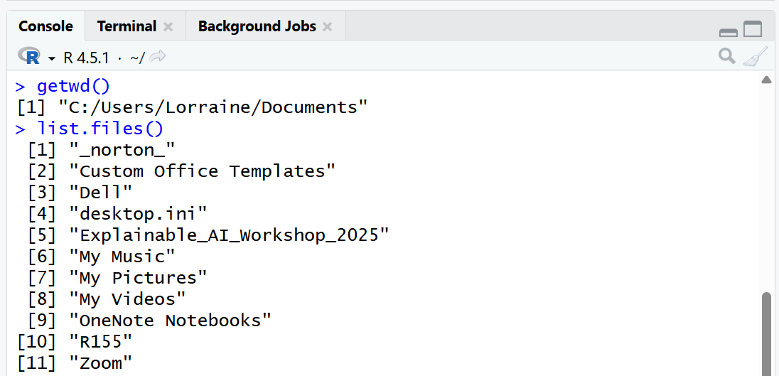
✅ Look at the output from getwd() and list.files() in the Console. Notice which folder R is using and which files R can see there. The folder may be different from the one containing chapter7_practice.Rmd. You will compare it with the knitted notebook output next.
🗣 When you run getwd(), you are checking where R is currently “looking.” When you run list.files(), you are checking what R can actually see from that location.
🧭 If the file you need is not listed, your next move is to check whether the file is in the right folder or whether the working directory is set to the folder location where the desired file is saved.
The notebook works differently when you Knit it. For the notebook setup used in this chapter, R starts a fresh session and uses the folder where the Rmd file is saved. Let’s see that in action!
R Notebook
Check your working directory in the Notebook
Step 1
🎯 Add a new code chunk with the same code as above.
# ⚡ Type this in your notebook
getwd()
list.files()Step 2
🧶 Test knit.
🎯 Click the Knit button at the top of the R Notebook editor pane. This will run all the code in your notebook from top to bottom in a fresh R session and create an HTML document as output.
Step 3
✅ Verify
Review the output under the getwd() and list.files() chunk in the resulting HTML.
✅ In the knitted notebook output, look directly under the getwd() and list.files() chunk. Confirm that the folder path matches where you saved chapter7_practice.Rmd. Then check whether the file list includes the notebook file itself.
You should see the files for this chapter listed in the output:
[1] "car_prices.xlsx" "chapter7_practice.Rmd" "Values_Transport_dplace.csv"🗣 When this notebook is knitted, R uses the folder where the Rmd file is saved as the working directory.
🪞 Reflect: Did R look in the same folder both times, or did the Console and Knit use different folders? Either result is okay. Explain what your result tells you about where R is looking. Why does this matter when importing files? This is Task 2 of the Practice Space at the end of this chapter.
🧭 Before loading data, use getwd() and list.files() to confirm where R is looking and what it can see. In the Console, that location may be different from the notebook folder. When you Knit the notebook used in this chapter, keeping the data files beside the Rmd file allows R to find them by file name.
🌳 In
Chapter 9: Git and GitHub, you will learn how to organize data files in a subfolder.
For the remainder of this chapter, we will use the workflow where you load data files that are in the same folder as your R Notebook. This is a common and simple way to manage your files.
Import in R
This section shows you how to prepare R to import datasets. You will (1) install the packages needed for this chapter one time, and (2) load those packages every time you start a new R session so your notebook can run from top to bottom when you Knit.
📦 Packages refresher
To import data, we will need to use functions from additional packages that are not part of the base installation of R. A package is a collection of functions, data, and documentation that extends the capabilities of R. You were first introduced to packages in Chapter 3 when you installed rmarkdown to run your R Notebook.
Installing Packages
You need to download the package before you can use it. You only need to install the package once. Packages will need to be updated from time to time.
🎯 Install the packages you need for this chapter as a one-time action.
🧭 Choose either installation method below. Both install the same packages, so use the method that helps you understand and verify what R is doing.
Method A: GUI
Bottom-right pane → Packages tab → Install → type the package name.
In the bottom-right pane, you will see a tab called “Packages.” This is where RStudio lists the packages you have installed. You can install packages by clicking the Install button.
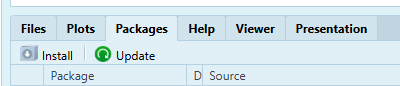
dslabs in the Packages box and click Install to download dslabs from the Package Repository CRAN🗣 After you click Install, notice the lines of code and message(s) that result in the Console. The code is what you would have to type if you were installing packages without using the GUI (Method B).
Method B: Type the code in the Console
Often, you will use the function install.packages() to install a package. This chapter uses readr to import CSV files, readxl to import Excel files, and dslabs to provide a curated dataset for practice.
🎯 Install the packages readr, readxl, and dslabs using install.packages().
# ⚡ Type this in your Console to install packages
install.packages("dslabs") # You can install one package at a time
install.packages(c("readr", "readxl")) # Or use c() to install multiple packages🗣 The install.packages() function installs packages from CRAN. Messages during installation are normal. Warnings are also common and are often not fatal, but read them and use packageVersion() to confirm that the package installed. An error means the installation did not complete successfully. This code installs the dslabs, readr, and readxl packages. The c() function combines the package names into a vector, allowing you to install multiple packages at once.
⚠️ Common Pain Point: Run
install.packages()in the Console rather than putting it in an R Notebook code chunk. If an installation line remains in the notebook, knitting may try to install the package again and will return an error when rendering files. Keep thelibrary()lines in the notebook so the packages load when the notebook runs.
# ✅ Check
packageVersion("dslabs")[1] '0.9.1'packageVersion("readr")[1] '2.2.0'packageVersion("readxl")[1] '1.5.0'✅ Each packageVersion() line should print a version number. A version number means the package is installed on your computer. If you get an error saying there is no package with that name, the package did not install successfully.
After installing packages, you need to load them into your R session to use their functions. This is done with the library() function, which we will cover next.
Loading Packages
After installing the package, you need to load it into your R session using the library() function. This makes the functions in the package available for use. Every time you start a new R session, you will need to load the packages you want to use. To ensure your R Notebook works when you Knit it, you should include the library() calls in your R Notebook.
💡 Tip: Add headings and format your report as you work. 🎯 Add the heading # Library Packages.
🎯 Load the packages readr, readxl, and dslabs into your R session using a notebook code chunk so they load each time you Knit. This is Task 3 of the Practice Space at the end of this chapter.
# ⚡ Type this in a code chunk in the R Notebook to load packages
library(dslabs) # For more datasets
library(readr) # For reading CSV files
library(readxl) # For reading Excel files🗣 library() may print startup messages, and those messages are not automatically a problem. A normal startup message provides information about the package or session. An error means the package did not load.
🧶 Test knit.
Your folder system, notebook, and packages are now set up to import data. The next step is to learn how to load different sources of tabular data.
Tabular data
Tabular data is data that is arranged in a table format where rows represent observations and columns represent variables. Rows usually represent observations (cases, people, states, experiments, etc.). Columns usually represent variables (measurements you recorded). This is the most common format for datasets and what most people think of when they think about data. When you import data into R, it is often stored as a data frame.
A data frame (df) is the most common way to store tabular data in R. It is a two-dimensional table made of rows and columns. Data frames are rectangular. Every column must have the same number of rows. In other words, each column must be the same length, because every row must have a value (or an NA) for every column. A data frame can store different data types in different columns (numbers, characters, logical values, etc.). A practical way to think about a data frame is a collection of columns, where each column is a vector.
This section shows two common ways to bring data into your R session.
You can load datasets that already come with R or with an installed package. These are fast and reliable for practice.
You can import data files from your computer, such as CSV or Excel files. These require the correct package, file name, and file path.
We will practice both in this chapter because future chapters will ask you to use built-in package data and imported data files.
Package Datasets
To load package datasets, use the data() function with the name of the dataset and the package it comes from.
📜 The basic SYNTAX: data("dataset_name", package = "package_name")
Base R Datasets
Base R comes with a set of built-in datasets that you can use for practice and learning. These datasets are part of the base R installation and are available without needing to install any additional packages.
🎯 View a list of datasets that are already in R
# ⚡ Type this in your Console to see the available datasets in base R
data(package = "datasets")🗣 This opens a list of datasets that come from R by default. You can see the name of the dataset and a brief description of it.
These datasets are already available, but you can make their availability more explicit by loading a selected dataset into your Environment with data(). In later chapters, we will often use mtcars from base R.
🎯 Load the mtcars dataset from base R. This is Task 4 of the Practice Space at the end of this chapter.
# ⚡ Type this in your R Notebook to load the mtcars dataset
data("mtcars")🗣 After running this code, the mtcars dataset is loaded into your R environment.
✅ Look in the Environment pane for mtcars. You can click the object in your environment to view the data. Alternatively, you can run the code View(mtcars). Either method will open a new window in RStudio that displays the data.
🧐 Notice: The
mtcarsdataset has row names, which are labels stored outside the regular data columns. Row names can be convenient for display, but they do not behave like a regular variable. In most projects, identifiers should be stored as a column instead.
🧶 Test knit.
Curated Datasets
In addition to the base R datasets, there are packages that you can install that provide additional datasets for practice and learning. These datasets are often curated and come with documentation that explains the context and variables in the dataset. One popular package is dslabs, which provides datasets for practice and learning in data science.
# ⚡ Type this in your Console to see what datasets are available from dslabs
data(package = "dslabs") 🎯 Load the movielens dataset from the dslabs package. This is Task 5 of the Practice Space at the end of this chapter.
# ⚡ Type this in your R Notebook to load the "movielens" dataset
data("movielens", package = "dslabs")🗣 The movielens dataset from the dslabs package is loaded into the R environment.
✅ You can click the object in your environment to view the data.
🌱 Chapter 8 will teach you how to explore tabular data in more detail.
🧭 If a dataset does not appear, your next step is to check the sequence of your notebook. Code that loads packages and data must come before code that uses those objects.
🧶 Test knit.
These datasets are great for practice, but in real projects, you will often need to import data from external files. The next section shows you how to do that.
External Files
Often, you will need to load data from external files that you have downloaded or created. The most common file formats for data are CSV (.csv) and Excel (.xlsx). To load these files into R, you will need to use functions from the readr and readxl packages, respectively.
Read CSV
Importing a CSV file with read_csv() requires the readr package, which you loaded earlier. If you forget to load readr with library(readr), R will report that it cannot find read_csv().
For the notebook setup used in this chapter, the CSV file is saved in the same folder as the Rmd file. When you Knit, this allows you to use only the file name in the import code.
📜 The basic SYNTAX:
df <- read_csv("file.csv")
🎯 Import the CSV file Values_Transport_dplace.csv into R using read_csv() and store it as dplace_df. This is Task 6 of the Practice Space at the end of this chapter.
# ⚡ Type this in your R Notebook to import the CSV file
dplace_df <- read_csv("Values_Transport_dplace.csv")🗣 The read_csv() function reads the CSV file and creates dplace_df, a data frame that contains the data from the CSV file.
✅ You can click on dplace_df in your Environment to view the imported data.
🧐 Notice: When loading, R prints an import summary to confirm what it found. The
dplace_dfdata frame contains 185 rows and 7 columns.Delimiter: ","means R detected a comma-separated file. The column specification shows howreadrinterpreted each column. In this case,chr (3)means 3 character columns:id,name, andsub_case.dbl (4)means 4 numeric columns:domainelement_pk,pk,valueset_pk, andyear.
🧶 Test knit.
🧭 If the import does not work, read the first line of the error message and check the most likely problem first.
- If the error says the file cannot be opened or does not exist, R cannot find
Values_Transport_dplace.csv.- Check the spelling, capitalization, underscores, and
.csvending. - Check that the file is in the same folder as your Rmd file.
- Check the spelling, capitalization, underscores, and
- If the columns look wrong, the file may not have been read as a comma-separated file.
- Make sure you did not open and resave the CSV file in Numbers or Excel.
- If you are unsure, delete the file and download a fresh copy.
- If the error says could not find function
read_csv, thereadrpackage is not loaded.- Run
library(readr)in a code chunk before the import code.
- Run
🛠 Break Things! Test a common error on purpose. Close and reopen RStudio, then run this line before running library(readr):
dplace_df <- read_csv("Values_Transport_dplace.csv")You should see an error saying R cannot find the read_csv() function. This does not mean the CSV file is broken. It means the package that contains read_csv() has not been loaded yet.
💡 Tip: Any time you reopen RStudio, run all code chunks to load your packages and data into R again.
Read Excel
Importing an Excel file requires the package readxl that we loaded earlier. If you did not load the readxl package, you will get an error message when you try to use read_excel().
Type read_excel() in your notebook
For the notebook setup used in this chapter, saving the Excel file in the same folder as the Rmd file allows you to use only the file name when you Knit.
df <- read_excel("file.xlsx")
🎯 Import the Excel file car_prices.xlsx into R using read_excel() and store it as car_prices_df. This is Task 7 of the Practice Space at the end of this chapter.
# ⚡ Type this in your R Notebook to import the Excel file
car_prices_df <- read_excel("car_prices.xlsx")🧐 Notice: Be patient when you load an Excel file. R may take a few seconds to read an Excel file, especially if the file is large, has complex formatting, or if you are importing more than one sheet. Very large Excel files can take longer to import. The limit is usually the computer’s available memory and processing power, not RStudio itself. However, opening a very large dataset in RStudio’s data viewer can slow down the RStudio window a lot.
🗣 The read_excel() function reads the Excel file and creates a data frame called car_prices_df that contains the data from the Excel file. You can click on car_prices_df in your environment to view the imported data.
💡 Tip: If the Excel import fails while the workbook is open in Excel, close the workbook and try the import again.
✅ Look in the Environment pane for car_prices_df. Click the object or run head(car_prices_df) to confirm that the rows and columns look like car price data.
View the data frame by clicking on car_prices_df in your Environment pane or by running View(car_prices_df) in your console.
🧭 If the Excel import does not look right, check three things before asking for help: whether the file is listed in list.files(), whether the file name is spelled exactly as car_prices.xlsx, and whether the workbook has more than one sheet.
🧶 Test knit.
🌳 Multiple Sheets
Excel files can contain multiple sheets. By default, read_excel() reads the first sheet. If your Excel file has multiple sheets, you can specify which sheet to read using the sheet argument. You can specify the sheet by name or by number.
# Optional Example
excel_sheets("car_prices.xlsx")
car_prices_sheet1 <- read_excel("car_prices.xlsx", sheet = 1)🗣 The excel_sheets() function lists the names of the sheets in the Excel file. The read_excel() function with the sheet argument reads the specified sheet from the Excel file.
🧭 When a workbook has multiple sheets, use excel_sheets() to inspect the available names, then select the sheet you need by number or name. For example, sheet = 1 selects the first sheet, while sheet = "car_prices" selects it by name.
🧶 Test knit.
Create RData file
This task creates an RData file.
🎯 Save the environment objects car_prices_df, dplace_df, movielens, and mtcars into a file called chapter7_practice.RData.
Run this code after car_prices_df, dplace_df, movielens, and mtcars exist in your Environment.
# ⚡ Type this in your R Notebook to save the selected objects in an RData file
save(
car_prices_df,
dplace_df,
movielens,
mtcars,
file = "chapter7_practice.RData"
)🗣 save() writes chapter7_practice.RData in the current working directory. When you Knit the notebook used in this chapter, that directory is the folder containing chapter7_practice.Rmd. After knitting, use list.files() or Finder or File Explorer to confirm that the RData file is there.
🧭 Saving selected objects gives you control over what the RData file restores later. Here, you are preserving the four objects used in this chapter rather than saving everything in the Environment.
Summary
In this chapter, you learned how datasets enter R and why file management is a common reason imports fail. We started by defining tabular data as a table where rows represent observations and columns represent variables. You also learned that imported tabular data is usually stored in a data frame, which is rectangular: every column has the same number of rows, and missing values should appear as NA.
You also learned how the working directory controls where R looks for files. You used getwd() to print the current working directory and list.files() to list the files R can see in that folder. You compared running code in the Console to knitting an Rmd file, where code chunks usually use the Rmd file’s folder as the working directory. To prevent “cannot open file” errors, you practiced saving downloaded data files in the same folder as your R Notebook and checking that the filenames appear in list.files() before importing.
Finally, you practiced the core import workflows introduced in this chapter. You installed packages with install.packages(), verified installation with packageVersion(), and loaded packages each session with library(). You loaded built-in and package datasets with data(), then imported external files with read_csv() for CSV files and read_excel() for Excel files. When something did not work, you used targeted checks for the working directory, file visibility, and loaded packages.
You now have a repeatable import workflow: place the file, check where R is looking, confirm R can see the file, load the right package, import the data, and verify the result. This workflow supports autonomy by helping you use evidence to choose a next step and ask a focused question when you need help.
Chapter Terms
Columns: The vertical fields in a data frame or table. In tidy tabular data, each column usually represents one variable, such as a name, category, measurement, count, or logical value. In R, each column in a data frame is a vector, and all columns must have the same number of rows.
CSV (Comma-Separated Values): A plain-text file (.csv) for rectangular (row-and-column) data where each row is a line and values are separated by commas. Because it’s plain text, CSV is widely compatible across software, but it does not reliably preserve spreadsheet features like formulas, cell formatting, or multiple sheets.
Data Frame: A two-dimensional R object for tabular data, organized as rows and columns. Each column is a vector (or factor) with the same number of rows, columns can have different data types, and the object has class “data.frame”.
Excel (.xlsx): A Microsoft Excel workbook file (.xlsx) that can store one or more worksheets, along with spreadsheet features like formulas and formatting. .xlsx uses the Office Open XML format (the “x” indicates an XML-based file without macros).
File Path: A text “address” that tells the computer (and R) where a file or folder is located. Paths can be absolute (the full location from the start of the file system) or relative (interpreted relative to your current working directory). In R, getwd() shows the current working directory that relative paths are based on, and file.path() helps build paths in an operating-system-safe way.
Graphical User Interface (GUI): A point-and-click interface that lets you interact with software using menus, buttons, and file browsers instead of typing commands. In RStudio, the Import Dataset wizard is a GUI tool that helps you select a file and then outputs the R code (including the file path) needed to reproduce the import, so you can copy that code into your R script.
Package: An installable collection of R code, including functions, documentation, and sometimes datasets, that adds new features beyond base R. Packages are commonly installed from CRAN and then loaded with library() so you can use their tools in your session.
Rows: The horizontal records in a data frame or table. In tidy tabular data, each row usually represents one observation, case, or unit being measured, such as one person, car, state, experiment, or survey response.
Tabular Data: Data arranged in a table (a rectangular structure) where rows represent records/observations and columns represent variables/attributes. This row–column layout is the standard format used by spreadsheets, databases, and data frames.
Working Directory: The folder on your computer that R treats as the default “home base” for the current session. When you read files (e.g., read.csv("data.csv")) or save outputs (e.g., write.csv(df, "results.csv")) using relative paths, R looks in (and writes to) the working directory unless you specify a full path. You can view or change it using Session → Set Working Directory, and you can check it with getwd() or change it with setwd("path/to/folder").
📝 Practice Space
In most chapters, the Guided Activity helps you create a notes file first, and then the Practice Space asks you to create a separate practice file.
Chapter 7 works differently because importing data is not only about typing the correct R function. Importing data requires understanding your folder structure and careful step-by-step verification and troubleshooting. For this reason, the Guided Activity helps you begin building the same chapter7_practice.Rmd file that you will use for this Practice Space.
You will need two data files for this chapter:
As you complete the Guided Activity, tidy the formatting and add memos to your chapter7_practice.Rmd file. The Practice Space below gives you a checklist of the tasks to complete.
- Complete Tasks 1–7 in your Rmd file. Each task includes one required Comment or Reflect memo.
- Task 8 reminds you to save the four selected objects in an RData file. It does not require a memo.
- Tasks 9–13 are multiple-choice self-check questions. They do not belong in your Rmd file. Complete them in the separate quiz provided through your course site.
By the end of this Practice Space, your Module_4 folder should contain:
Intro_to_R/
└── Module_4/
├── chapter7_practice.Rmd
├── chapter7_practice.nb.html
├── chapter7_practice.RData
├── Values_Transport_dplace.csv
└── car_prices.xlsxSome workflows create chapter7_practice.html instead of chapter7_practice.nb.html.
Your R environment should contain:
mtcarsmovielensdplace_dfcar_prices_df
In Tasks 1–7, you will see two kinds of required memo prompts:
- 🗣 Add Comments asks you to explain what the code, output, or result shows.
- 🪞 Reflect asks you to explain your learning process or understanding, including what confused you, what changed, or what strategy you would use next.
Answer the Comment or Reflect prompt included in each task. Keep the memo short and useful. One to three thoughtful sentences is enough.
Whenever a human or digital resource contributes to your work, add a 👀 Cite memo. Identify the resource and explain how it helped.
🧭 Show autonomy by checking your file locations, reading your output carefully, using error messages as evidence, and explaining what you would check next if something did not work.
If you encounter an error, add a short memo that records what happened, what you checked or changed, and what still confuses you. If a resource helped, include a 👀 Cite memo.
Follow the AI-use guidance that applies to your learning setting. If you use an AI tool, add a 👀 Cite memo naming the tool and explaining what it contributed. Clearly mark any words you reproduce exactly as quoted text, using quotation marks or a block quote with >.
Task 1
🗂 Organize your files
🎯 Download the two data files for this chapter and place them in the same folder as your R Notebook.
Files for this chapter:
Values_Transport_dplace.csvcar_prices.xlsx
✅ Check your folder in Finder or File Explorer. You should be able to see your Rmd file and both data files together in the same folder.
🗣 Add Comments: Explain why keeping the Rmd file and the data files in the same folder makes importing data simpler in this chapter.
Task 2
📁 Check where R is looking
🎯 Run getwd() and list.files() in the Console. Then include the same code in a code chunk of your R Notebook and 🧶 knit the notebook.
Step 1
Type and run this code in the Console first.
# ⚡ Type this in the Console
getwd()
list.files()Step 2
Add a code chunk in your R Notebook, write the same code in that code chunk, then 🧶 knit your notebook.
# ⚡ Type this in your notebook
getwd()
list.files()
Step 3
✅ Check the resulting HTML and compare with Console output.
🪞 Reflect: Did R look in the same folder both times, or did the Console and Knit use different folders? Either result is okay. Explain what your result tells you about where R is looking. Why does this matter when importing files?
Task 3
📦 Load packages
🎯 Load the packages readr, readxl, and dslabs into your R session.
# ⚡ Type this in your R Notebook. Fill in the blanks.
_______(readr)
_______(readxl)
_______(dslabs)
✅ The library() lines should run without an error. Then use packageVersion() for each package to confirm that it is installed.
# ✅ Check
_______(_______)
_______(_______)
_______(_______)
🗣 Add Comments: Explain the difference between installing a package one time and loading a package each time you start a new R session.
Task 4
🚗 Load a Base R dataset
🎯 Load the mtcars dataset from base R.
# ⚡ Type this in your R Notebook. Fill in the blanks.
_______(_______)
✅ Check that mtcars loaded correctly.
# ✅ Check
head(mtcars)
🗣 Add Comments: Explain why mtcars can be loaded with data() instead of imported from a file on your computer.
Task 5
🎬 Load a curated package dataset
🎯 Load the movielens dataset from the dslabs package.
# ⚡ Type this in your R Notebook. Fill in the blanks.
_______(_______, package = "_______")
✅ Check that movielens loaded correctly.
# ✅ Check
head(movielens)
🗣 Add Comments: Explain what the package = "dslabs" part tells R to do.
Task 6
📄 Import a CSV file
🎯 Import the CSV file Values_Transport_dplace.csv into R using read_csv() and store it as dplace_df.
# ⚡ Type this in your R Notebook. Fill in the blanks.
dplace_df <- _______(_______)
✅ Check that the data imported correctly.
# ✅ Check
dim(dplace_df)   # should print 185 7
head(dplace_df)
🪞 Reflect: Explain how you knew the CSV import worked. Use evidence from the import summary or your checks, such as the number of rows and columns, the comma delimiter, or the column types. Then name one likely cause of an error if this import failed: the file was not in the same folder as the Rmd file, the file name was typed differently, or library(readr) had not been run.
Task 7
📊 Import an Excel file
🎯 Import the Excel file car_prices.xlsx into R using read_excel() and store it as car_prices_df.
# ⚡ Type this in your R Notebook. Fill in the blanks.
car_prices_df <- _______(_______)
✅ Check that the data imported correctly.
# ✅ Check
dim(car_prices_df)   # should print 10000 16
head(car_prices_df)
🪞 Reflect: Explain how importing an Excel file is similar to and different from importing a CSV file. Name the package/function used for the Excel file, explain why the file can be imported with only "car_prices.xlsx" instead of a longer file path, and describe one thing you would check if the import failed or the data did not look right.
Task 8
💾 Save selected objects in an RData file
🎯 Save the four selected objects in a file called chapter7_practice.RData.
This file should contain:
car_prices_df(the data frame created by importing the Excel file)dplace_df(the data frame created by importing the CSV file)movielens(the data frame created by loading the dataset from thedslabspackage)mtcars(the data frame created by loading the dataset from base R)
# ⚡ Type this in your R Notebook
save(
  car_prices_df,
  dplace_df,
  movielens,
  mtcars,
  file = "chapter7_practice.RData"
)
✅ Check that the .RData file was created and is saved in your module folder.
Finish and verify your notebook
🎯 Step 1: Clear your Environment.
Click the 🧹 broom icon in the Environment pane to remove the current objects.
🎯 Step 2: Run the notebook from top to bottom.
Use Run → Run All to execute every code chunk in order. The code in your notebook should recreate mtcars, movielens, dplace_df, and car_prices_df before saving them in chapter7_practice.RData.
🎯 Step 3: Save, knit, and inspect.
Save the .Rmd file and knit it to HTML. RStudio will usually create a .nb.html file for an R Notebook, although some workflows create a .html file.
✅ Open the HTML output and confirm that it includes the expected headings, code, output, and memos. Check your module folder and confirm that the Rmd, HTML, RData, CSV, and Excel files are present.
Multiple-choice self-check
Tasks 9–13 do not belong in chapter7_practice.Rmd. Complete these questions in the separate quiz provided through your course site.
Choose the best answer for each question.
Task 9
Which statement best defines tabular data?
A. A list where each element can be a different length
B. A table where rows represent observations and columns represent variables
C. A single vector that stores only numbers
D. A plot with x- and y-axes
Task 10
list.files()What does the output tell you?
A. Which packages are installed on your computer
B. Which functions are available in Base R
C. Which files are in R’s current working directory
D. Which objects are stored in the Environment pane
Task 11
You click Knit and get an error that a file cannot be opened. What is the best first check?
A. Reinstall R and all packages
B. Run getwd() and list.files() to confirm where R is looking and whether the file is there
C. Prompt an LLM with the error message to get suggestions for how to fix it
D. Rename the file to something shorter
Task 12
Which function is used in this chapter to import an Excel .xlsx file?
A. read_csv()
B. read_excel()
C. readxl()
D. readr()
Task 13
Which function is used in this chapter to import a CSV file?
A. read_csv()
B. read_excel()
C. readxl()
D. readr()