Chapter 5 Help!

Using R Help Files to Troubleshoot Knit Errors

Overview

Chapter 5 focuses on making your R Notebook organized, reproducible, and shareable.

You will learn how to use Markdown and YAML to structure your notebook, then knit it into an HTML report that someone else can read without opening RStudio. You will also practice using R help files to understand functions, arguments, and examples.

The main goal of this chapter is to build confidence with the normal problem-solving process in R. Instead of trying to memorize everything, you will learn how to use help resources and document what you learned in a shareable report.

In this chapter, you will practice how to:

#️⃣ Format your R Notebook using Markdown headings.
🧾 Add basic document information in the YAML header.
📤 Knit an R Notebook into a shareable HTML report.
⚠️ Recognize common reasons a notebook fails to knit.
🛠 Use error messages and help files to troubleshoot problems.
🔎 Open and read R help pages for functions.
🧮 Identify required arguments and default arguments.
✅ Use help pages to solve a problem with missing values.
🦁 Practice deciding when to keep troubleshooting, when to change strategies, and when to ask for help.

R Notebook -> HTML Report

In this chapter, you will learn how to turn your R Notebook into a shareable HTML report. The report records both your results and the process you used to reach them. 🦁 Courage in this chapter means staying engaged when an error or unfamiliar help page creates uncertainty, using the evidence to choose a reasonable next step, and asking for help before the struggle becomes unproductive. The chapter models this process, and the Practice Space asks you to use it and document what you tried and learned.

🎯 Please open a new R Notebook and save it as chapter5_notes.Rmd in the folder you use for this chapter. Use this document to take notes and practice the chapter content.

Open RStudio → File → New File → R Notebook.
Save it in the folder you use for this chapter as chapter5_notes.Rmd.
Keep the YAML header at the top of the notebook. Delete only the sample body text and example code below the second --- line.

🧐 Notice: The YAML header is the block between the two --- lines at the top. Keep that block because it controls the notebook’s title and output format.

In the YAML header, update the title to match this chapter. The next section explains how to add a date.

YAML Date Field

The YAML header is the metadata “label” for your notebook. It controls document settings like the title, date, and output format.

Good document labels help future-you and anyone who reviews or continues the work understand what the file is, when it was created, and what kind of output RStudio should build. This is a small documentation habit, but it matters when you are trying to keep your work organized.

A basic YAML header looks like this:

---
title: "R Notebook"
output: html_notebook
---

🎯 Add a date to your notebook by editing the YAML header to include a date: field.

Method A. Hard Code

Manually type the date you created the notebook. Include quotation marks around the date.

---
title: "Chapter 5 Notes"
date: "May 25, 2026"
output: html_notebook
---

Method B. Dynamic Date

Use R code to generate the current date automatically each time you knit the document. The inline R expression `r Sys.Date()` retrieves the current date from your computer’s operating system. This follows the syntax: backtick (`), then r, a space, Sys.Date(), and a closing backtick (`). The backtick is located above the Tab key on most keyboards.

---
title: "Chapter 5 Notes"
date: "`r Sys.Date()`"
output: html_notebook
---

Inline R works in YAML when written exactly as shown above. Notice the backticks around `r Sys.Date()` and the quotation marks around the complete expression: date: “`r Sys.Date()`”. You can learn more about inline R in the 📝 Notebook Advanced Activity, but for now, you can copy and paste the above YAML section to add a dynamic date to your YAML header. Each time you knit the document, the date will update to the current date.

You’ll learn how to knit soon, but first, you need a clear structure inside the document. That is where Markdown headings come in.

Heading levels

Headings create the outline of your notebook. The number of # symbols controls the heading level.

# Biggest heading

Text here will be in paragraph font.

## Main section heading

Text here will be in paragraph font.

### Subsection heading

Text here will be in paragraph font.

The chapter HTML pages in this book were created using RStudio. Notice how headings create a structured outline and how font sizes change with each heading level.

🎯 Add headings to your Chapter 5 Notes.

# Notebook set up

[Add any memos or notes here to help you remember how to set up your notebook, such as how to add a date to the YAML header.]

## Markdown structure

[Add any memos or notes here to help you remember how to format and navigate your report in RStudio.]

## Knit to HTML

# Built-in Functions

## Help Files

🎯 Work to complete the sections under each heading as you go through the chapter content. You can also add more headings and subheadings as needed to organize your notes and code.

Outline Menu

The “outline pane” in RStudio uses your Markdown headings to create a clickable map of your document. This document outline or outline menu in the Source pane shows your headings/subheadings. They act as “Jump To” menus, helping you move between tasks without scrolling through the whole notebook.

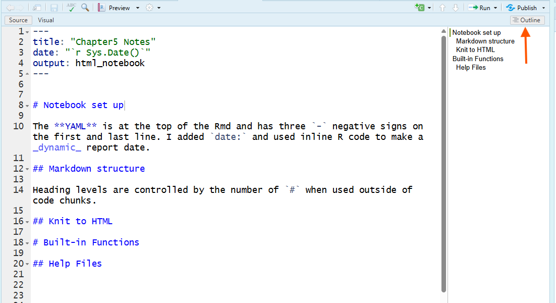
Figure 1. Screenshot of R Markdown formatting

Figure 1 shows an RStudio R Notebook with a Markdown section heading (for example, ## Markdown structure) in the editor and the Outline menu on the right. Markdown headings create the structured outline. The orange arrow points to the Outline button used to show or hide it. 💡 Tip: Clicking a heading in the Outline menu jumps to that section in the report.

In this example, # Notebook set up creates a main section heading.

The most common beginner mistake with `#`

Put a space between the # symbols and the heading text to ensure the heading formatting works correctly.

For example, ##Task 1 will not format as a heading, but ## Task 1 will.

The # symbol means two different things depending on where you type it.

Outside a code chunk, # creates a Markdown heading.

🎯 Type ### Task 1 under ## Markdown structure to create a subsection heading.

## Markdown structure

Heading levels are controlled by the number of `#` symbols when they are used outside code chunks.

### Task 1

Inside a code chunk, # creates an R comment. R ignores the comment when it runs the code.

🎯 Type # This is a comment inside a code chunk. inside a code chunk to create a comment. 💡 Tip: Click the Insert Chunk button in the toolbar (green C with plus sign) and choose R from the drop-down list.

## Markdown structure

Heading levels are controlled by the number of `#` when used outside of code chunks.
Compare what you typed with the image of the knitted result.

### Task 1

🎯 Make a comment inside a code chunk

```jeo
# ⚡ This is a comment inside a code chunk.
cursed_seq <- c(4, 8, 15, 16, 23, 42)
```

🗣 The `#` symbol has two different meanings in R Notebooks.

🧐 Notice: To write notes about your code, type # inside the code chunk. Write result memos and learning reflections outside the code chunk without #.

Now that you have the basics of Markdown structure, you will test whether the whole notebook is ready to become an HTML report.

Knit to HTML

When you 🧶Knit to HTML, RStudio creates a static report file that includes your formatted headings and text, your code, and the output produced when the code runs. RStudio saves the HTML file on your computer and opens it in a web browser. Opening the file in a browser does not publish it on the internet. The browser address points to a file on your computer, so another person cannot use that address to open your report. To share the report, send or upload the .html file itself.

Knitting is not the same as “running a chunk.” Running a chunk uses your current R session. This means that running a code chunk can succeed even if you wrote code out of order or if objects used already exist in your Environment.

Knitting is a stronger test. It runs the entire notebook from top to bottom in a fresh session, then builds an HTML report.

How to Knit

RStudio interfaces vary. You may have a 🧶Knit button, or you may see a Preview drop-down menu.

Option 1: Knit button

In the Source pane, click the Knit button (it looks like a ball of yarn with a knitting needle 🧶).

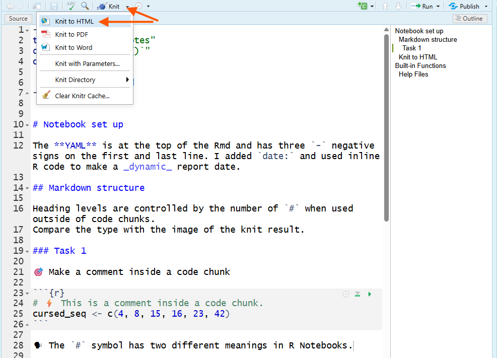
Figure 2 is a screenshot of RStudio showing the 🧶Knit button on the toolbar (highlighted by an orange arrow), which students can click to knit the R Notebook into an HTML document.

Option 2: Preview menu

In the Source pane, click the Preview drop-down menu and select Knit to HTML.

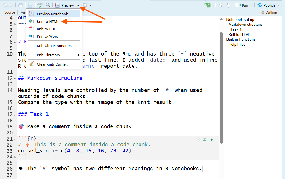
Figure 3 is a screenshot of RStudio with the Preview menu opened; orange arrows highlight the Preview dropdown button and the Knit to HTML option, showing how to knit an R Notebook into a shareable HTML document (not just run a single code chunk).

Below is the result you get after knitting to HTML.

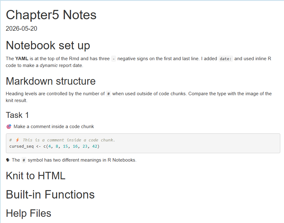
Figure 4. Screenshot of resulting HTML report

Figure 4 is a screenshot of the knitted HTML output in a web browser showing the notebook title (“Chapter5 Notes”), the subsection heading (“Task 1”), memos as regular paragraph text, and an R code chunk, demonstrating what you get after you Knit to HTML.

When you knit, RStudio automatically does three things:

Starts a fresh R session (your Environment does not count).
Runs your notebook from top to bottom in order.
Produces an HTML file you can view and share.

This is why knitting is the real test of “does this notebook work?” If it knits, someone else (including future-you) can see the workflow and results without needing to open RStudio.

✅ Check: Your notebook must create every object it uses in the notebook itself. Your Environment does not count. Knitting may reveal a code error you did not notice. That is useful information about the first place in your workflow that needs attention.

Knit Errors

When you knit, the Render tab shows progress messages as R runs your notebook from top to bottom.

A successful knit has three visible signs:

The Render tab shows the process finishing without an error message.
Your notebook opens as a formatted web page in a browser window or in RStudio’s Viewer.
An .html file appears in the same folder as your .Rmd file.

🦁 Courage: A failed knit can feel frustrating or uncertain. Courage does not require you to ignore that feeling. Read the error, use it as evidence, and take one informed next step.

Read the error message in the Render tab.
Find the line or chunk that caused it. The error usually names a chunk or shows a line number.
Fix the first error you see. Many later errors are just “domino effects.”
Knit again.

✅ Check: A knit error is a “not yet” signal. What specific problem is R naming, and what evidence can guide your next step?

Common reasons knitting fails:

You wrote the code out of order, so an object exists in your Environment but is not created earlier in the notebook.
You forgot to include setup code, such as loading packages, creating objects, or reading files through the appropriate relative paths.
A chunk contains an error you did not notice because you never ran that chunk.

If Pandoc says the .knit.md file does not exist

RStudio uses a converter called Pandoc after R runs the notebook. If the Render tab first says output file: filename.knit.md and then says that the same .knit.md file does not exist, try this simple reset first:

Save your .Rmd file and close RStudio.
Check that the .Rmd file is still in your Chapter folder. If you also see a file ending in .nb.html, delete only that file. Windows may show it as chapter5_notes.nb and label it Chrome HTML Document.
Reopen the .Rmd file and knit again. RStudio can create a new .nb.html file if it needs one.

Do not delete the .Rmd file. That is the file containing your work.

If the error continues:

Save a copy of the .Rmd file in a short, local folder path that is not inside OneDrive, another cloud-synced folder, a network drive, or a downloaded ZIP file. On Windows, an example is C:/Users/YourName/DATA-R155/Chapter5/.
Close RStudio, reopen the copied file from that folder, and knit again.
If it still fails, create the small setup_check.Rmd document from the Check Your Installation section in the same local folder and knit it.
If the setup check also fails, stop and ask for help. Send the complete Render tab text and run the following lines in the Console so you can include the results:

R.version.string
R.version$arch
RStudio.Version()$version
rmarkdown::pandoc_version()
rmarkdown::find_pandoc()

If Settings > System > About > System type says ARM-based processor, include that fact. The instructor may need to check whether your computer should use the Windows emulation setup for RStudio or the native ARM64 version of Positron. Do not install a separate copy of Pandoc or Quarto, change Windows emulation settings, or disable security software as a first step.

🦁 Courage: Know when to ask for help. If you have made two focused attempts or spent about 10 minutes without learning anything new, stop repeating the same strategy. Save the exact error message and the smallest relevant code chunk. Note what you tried, then ask a peer, instructor, tutor, or another appropriate resource for help.

Next, you will shift from building the report to writing code inside it.

💡 Tip: Knit after any meaningful formatting or code change. It is easier to find an error when it was caused by your most recent edit.

Built-in Functions

Now that your notebook can become an HTML report, you need code worth documenting inside it.

Many built-in summary functions take a whole vector as input and return one summary value, or a small set of values. These are summary functions because they reduce many values down to a smaller result.

In this section, you will practice calling a function and noticing the difference between the stored function object and the function call that actually runs.

Function Objects vs. Function Calls

A function object is an R object that performs a task when it is called. For example, mean is the function object used to calculate the average of a numeric vector.

🎯 Run mean in a code chunk to see the stored function object. Add the code chunk under # Built-in Functions.

# ⚡ Type mean in your R Notebook inside a code chunk
mean

function (x, ...) 
UseMethod("mean")
<bytecode: 0x7681e15cb0>
<environment: namespace:base>

🗣 R displays the definition of the mean function object.

🦁 You do not need to understand every detail yet. For now, notice that typing mean without parentheses displays the function instead of calculating a mean.

To make the function do its job, you have to call it. A function call runs the stored code. To call a function, you type the function name followed by parentheses (). Inside the parentheses, you must provide any required arguments. For example, to calculate the mean of a numeric vector, you call the mean() function and provide the vector as an argument. The vector is a required argument because the function needs it to perform the calculation.

📜 The SYNTAX (basic):

mean(x)

where x is the numeric vector you want to summarize.

🎯 Calculate the mean of the cursed sequence.

# 📖 Review
cursed_seq <- c(4, 8, 15, 16, 23, 42)  

mean(cursed_seq)

[1] 18

🗣 The mean() function calculates the average of the numbers in the cursed_seq vector by summing them up and dividing by the count of numbers.

Help Files

Nobody memorizes every function or every argument. Looking in help is one way you stay engaged when you do not already know what to do or you have a question. Skilled R users look things up.

Typing a question mark before a function name opens its help file. For example, ?mean opens the help file for the mean() function. The Files pane usually contains several tabs, including the Help tab, which displays documentation for R functions.

🎯 Use ?mean to open the help file for the mean() function. Add the code chunk under ## Help Files.

# ⚡ Type this in your R Notebook
?mean

🦁 Test knit: If knitting fails, follow the Knit Errors steps and stopping rule.

🚀 Explore and Play: As we move through the remainder of the chapter, add meaningful headings and subheadings to your notebook to organize your notes and code as you wish.

No Required Arguments

Some functions do not have a required argument. For example, the Sys.Date() function returns the current date without needing any input.

🎯 Call the Sys.Date() function to get the current date from your computer’s operating system.

# ⚡ Type this in your R Notebook
Sys.Date()

[1] "2026-10-10"

🗣 The Sys.Date() function retrieves the current date from the system clock and returns it as a Date object.

🎯 Open the help file for the Sys.Date() function.

# ⚡ Type this in your R Notebook
?Sys.Date

🗣 The Sys.Date help page opens in RStudio’s Help tab. Note that Sys.Date() has no required arguments.

Scroll through the help file to find information about the function’s usage, arguments, and examples.

Usage: shows the function signature and defaults.
Arguments: what each argument does.
Examples: copy/run examples to learn patterns.

Sys.Date() is a friendly first example because it does not require an input. Most functions you use for data analysis will need at least one argument. Next, you will compare this to mean(), which needs a vector to summarize.

Required Arguments

Required arguments are the inputs a function needs to do its job.

🎯 Open the help file for the mean() function. Scroll through the help file to find information about the function’s usage, arguments, and examples.

# ⚡ Type this in your R Notebook
?mean   
help(mean)

🗣 The mean help page opens in RStudio’s Help tab. mean.default(x, trim = 0, na.rm = FALSE, ...) shows that x is a required argument, while trim and na.rm have default values.

Default Arguments

Default arguments are inputs with preset values that a function uses when you do not provide your own values. For example, the trim argument in the mean() function allows you to exclude a certain percentage of the lowest and highest values before calculating the mean.

The SYNTAX (with one default argument):

mean(x, trim = 0)

If you do not specify a value for trim, R uses the default value of 0, which means no values are excluded.

🎯 Calculate the trimmed mean of the cursed sequence, removing 20% of the lowest and highest values before computing the mean.

# ⚡ Type this in your R Notebook
mean(cursed_seq, trim = 0.2)  # drop 20% from each end first

[1] 15.5

🗣 The mean() function first removes 20% of the lowest and highest values from the cursed_seq vector, then calculates the mean of the remaining values. With 6 values and trim = 0.2, R trims 4 and 42, then averages 8, 15, 16, and 23.

✅ Check: How can you tell which arguments are required?

The main clue that x is required is that it has no = sign or default value next to it in the usage section. The other arguments have = signs, showing the default values that R will use if you don’t provide your own.

Some functions use ... (dot-dot-dot). That means “additional optional arguments may be allowed,” not required ones. For now, ignore ... until you are more advanced.

📜 Argument clue:

no = → usually required
= → R has a default value
... → extra optional arguments may be allowed; ignore this for now

🦁 You do not need to understand the whole help page before you can use one useful part of it.

Reading R Help Pages

Help pages are useful, but they are not written like beginner tutorials. They are written like reference pages. That means you need to learn where to look when you are trying to write, fix, or explain code. This section gives you a reading strategy for reading the help pages.

Open Help Page

If you know the function name, type a question mark before the function name.

# ⚡ Type this in your R Notebook
?mean

You can also use the help() function.

# ⚡ Type this in your R Notebook
help(mean)

🗣 The help page usually opens in the help tab in the bottom-right area of RStudio. That area contains several tabs, such as Files, Plots, Packages, Help, and Viewer.

Reading Order

When you open a help page, use this reading order:

Description: What does this function do?
Usage: What does the function call look like?
Arguments: What goes inside the parentheses?
Examples: What is one working pattern I can test?

For now, you may skim or skip sections like Details, Value, References, and See Also.

The Usage Section

The Usage section shows the basic recipe for writing the function call.

Open the help page for mean().

# ⚡ Type this in your R Notebook
?mean

In the Usage section, you may see something like this:

## Default S3 method:
mean(x, trim = 0, na.rm = FALSE, ...)

Read the usage line like this:

Part	What it means
`mean()`	This is the function being called.
`x`	Required. This is the object you want R to average.
`trim = 0`	Optional. R uses `0` unless you choose a different value.
`na.rm = FALSE`	Optional. Missing values are not removed unless you choose `TRUE`.
`...`	Extra options may be allowed. Ignore this for now.

In summary:

a required argument is an input the function needs before it can do its job.
a default argument is an input R already has a value for. You can use the default value, or you can replace it with your own value.

🗣 In mean(x, trim = 0, na.rm = FALSE, ...), the argument x is required because it does not have a default value. The arguments trim and na.rm are optional because R already has default values for them.

Use the Help Page to Solve a Problem

Let’s use the help page for a troubleshooting task. We’ll create a vector with a missing value, try a calculation, notice an issue with the result, and then use the help page to decide which argument needs to change.

🎯 Create a vector with one missing value.

# ⚡ Type this in your R Notebook
messy_scores <- c(80, 90, NA, 100)

print(messy_scores)

[1]  80  90  NA 100

🗣 The third position is marked with NA, which means the numeric value is missing.

🎯 Try to calculate the mean of messy_scores using only default arguments.

💬 Prediction: What do you think R will return? Calculate your predicted answer before you run the code.

# ⚡ Type this in your R Notebook
mean(messy_scores)
class(messy_scores)

🗣 R returns NA because the vector contains a missing value. By default, mean() does not remove missing values before calculating the average. This means that R cannot calculate the mean of the vector due to the missing value.

🦁 We haven’t yet learned how to change that behavior. This is the moment to use the help page.

🎯 Open the help page for mean().

# ⚡ Type this in your R Notebook
?mean

✅ Check: In the Arguments section, find the argument named na.rm.

🦁 Ask yourself:

What does na.rm control?
What default value does R use?
What value should I use if I want R to remove missing values?

🎯 Try the code again using na.rm = TRUE.

# ⚡ Type this in your R Notebook
mean(messy_scores, na.rm = TRUE)

[1] 90

🗣 The argument na.rm = TRUE tells R to remove missing values before calculating the mean. This does not delete the missing value from your original vector. It only tells mean() how to handle the missing value during this calculation.

Next, you will see how help-page examples can give you working patterns even when they do not exactly match your task.

Examples

The Examples section is often one of the most useful parts of a help page. Examples show working patterns. Your job is to adapt the pattern to your own object.

You are using the example to understand a structure, then applying that structure to your own task.

🎯 Run R’s built-in examples for mean().

# ⚡ Type this in your R Notebook
example(mean)

🗣 The example() function runs examples from the help page. You do not need to understand every line.

🦁 Help-page examples may look unfamiliar. Look for one pattern that helps you understand how the trim argument is used in the mean() function.

Unknown Function Name

So far, we knew the function name: mean().

Sometimes you know the topic, but you do not know the function name. For example, you might know you need help with missing values, but you may not know which function or argument to search for. In that case, use ?? or help.search().

🎯 Search for help pages related to “missing values” using ?? and help.search().

# ⚡ Type this in your R Notebook
??"missing values"

# ⚡ Type this in your R Notebook
help.search("missing values")

🗣 Use a pattern such as ?mean when you already know the function name. Use ??"search words" or help.search("search words") when you know the topic but not the exact function.

Situation	What to type
I know the function name.	`?mean`
I know the function name and want another option.	`help(mean)`
I know the topic but not the function name.	`??"missing values"`
I want to search help pages for a phrase.	`help.search("missing values")`
I want to run built-in examples.	`example(mean)`

Document Help

Troubleshooting is part of working in R. Documenting your troubleshooting efforts makes that work visible. When you use a digital or human resource, document where you went, why, and what you discovered.

🎯 Add a short help note to your report.

Type the 👀 Cite, 🗣 Comment, and 🪞 Reflect statements as regular Markdown text. Put only runnable R code and R comments inside the code chunk.


👀 I used `?mean` to read about the `na.rm` argument.

🗣 The help page showed that `na.rm` defaults to `FALSE`. 
I changed `na.rm` to `TRUE` because my vector contained an `NA` value.

# ⚡ Code
messy_scores <- c(80, 90, NA, 100)
# ✅ Check
mean(messy_scores, na.rm = TRUE)

[1] 90

🗣 The result is `90` because R averaged `80`, `90`, and `100` after removing `NA` from the calculation.

🪞 I learned that a default argument can be optional but still important. 
In this case, `na.rm` had a default value, but I needed to change it for my data.

🦁 If knitting fails, follow the Knit Errors steps and stopping rule.

🦁 Documenting your process of thinking helps you identify your understanding. It will increase self-awareness and help you regulate your cognitive processes. It will also help you prepare to ask for help when you need it. You will be able to show what you tried, what you learned, and what you need help with.

Summary

In this chapter, you strengthened your R Notebook habits by learning how to create a complete, shareable HTML report. You practiced editing the YAML header, using Markdown headings to organize your notebook, knitting your work to HTML, and sharing the actual .html file rather than a local browser address.

You also learned that knitting is the real test of whether your notebook works. Running a single chunk only checks part of the code in your current R session, but knitting runs the whole notebook from top to bottom in a fresh session. When knitting fails, the error message is feedback that helps you find what needs to be fixed next.

Finally, you learned how to use built-in R functions and help files. You practiced the difference between a function object and a function call, identified required and default arguments, used ?mean, help(), example(), and help.search() to find information, and changed na.rm = TRUE to handle missing values in a calculation.

Your main takeaway is that strong R work depends on organized notebooks, successful knitting, and the courage to use errors and help files as part of the coding process.

Chapter Terms

Arguments: Inputs that you provide to functions to customize their behavior. Arguments are specified within the parentheses of a function call and can modify how the function operates or what data it processes.

Default Arguments: Inputs that already have a preset value in the function definition and are used automatically when you don’t provide your own (e.g., mean(x, na.rm = FALSE) by default).

Examples Section: The part of an R help page that shows runnable code examples for how a function is used in practice. This section is often the fastest place to learn because it shows the function in context: what inputs go inside the function call, what the code looks like, and what kind of output to expect. In R, many help-page examples can also be run with the example() function.

Function Call: The act of running a function by writing its name followed by parentheses, optionally supplying arguments inside (e.g., mean(x)).

Function Object: A function stored as an R object (functions are “first-class” in R, meaning you can assign them to names, pass them to other functions, and inspect them).

Help Page: Documentation for R functions and packages that provides information on usage, arguments, and examples. For example, use ?mean or help(mean) to open the help page for mean().

Help Tab: Located in the Files/Plots/Packages/Help pane, this tab provides access to R documentation, package vignettes, and search functionality to find help topics related to R functions and packages.

HTML: A web page file type (.html) written in HyperText Markup Language that a web browser can open and display as a formatted document. Preview, Knit, or Render can create an HTML file (often .html or .nb.html) that shows your notebook’s text, code, and output. When the file opens from your computer, the browser address is a local file path, not a public link. Share the .html file itself.

Inline Code: Code-style text placed within a sentence by surrounding the text with single backticks, such as penguins. In Quarto and Markdown, inline code is used to mark object names, function names, file names, or short code expressions so they appear in a monospace code font in the rendered report. This formatting signals to the reader, “treat this as code or a code-related name,” not as ordinary prose.

Inline R: A short R expression written inside backticks with the prefix r (for example, `r Sys.Date()`) that is evaluated when you knit/render the document and replaced with its result in the output. Inline R is used to insert dynamic values (dates, computed statistics, labels) directly into your narrative text, and it can also be used in YAML fields like date: “`r Sys.Date()`” when supported.

Knit: In RStudio, the action that renders an .Rmd (including an R Notebook) into a finished output file (such as HTML, PDF, or Word) by running the document’s code chunks, inserting their results, and converting the document to the chosen format. Clicking the Knit button typically calls rmarkdown::render() in a new, clean R session, so everything needed to reproduce the result must be created or loaded in the document itself, and the output file is saved alongside the .Rmd.

Knit Button: The toolbar button in RStudio that renders an R Markdown file (.Rmd) into a finished output (e.g., HTML, PDF, Word) by calling rmarkdown::render() and running the document’s code to generate results. The output file is saved next to the .Rmd (same base name), and the button’s drop-down lets you choose among available output formats (shortcut: Ctrl/Cmd + Shift + K).

Outline Menu: A navigation tool in RStudio that uses your Markdown headings to create a clickable map of an .Rmd or .qmd document. The outline shows the structure of the notebook by heading level, so you can jump between sections without scrolling through the whole file. In RStudio, open it from the Outline button/menu in the Source pane toolbar.

Render Tab: A temporary tab that appears in RStudio’s Console pane when you Knit or Render an R Markdown (.Rmd) or Quarto (.qmd) document. It shows progress messages, warnings, and errors separately from your interactive Console, and typically includes a Stop control so you can interrupt a failed or long render.

Required Arguments: Inputs a function needs because they have no default value in the function definition; you must supply them in the call (or the function can’t do its job).

Usage Section: The part of an R help page that shows how to write the function call, including its arguments and any default values.

YAML Header: The metadata section at the top of an R Markdown or Quarto document, written between --- lines, that controls document settings like the title, author, date, output format (HTML/PDF/Word), and options for rendering.

📝 Practice Space

This Practice Space has two parts.

First, you will answer short multiple-choice questions that check whether you can organize an R Notebook, read an R help page, use a function argument, and explain why knitting is an important reproducibility check.

Second, you will practice troubleshooting an R Markdown file. Use the error messages and the troubleshooting workflow from this chapter to decide what to check and change.

Part 1: Check your understanding

Choose the best answer for each question in this section.

Task 1

🧾 YAML header

Which YAML header is the best match for a Practice Space Notebook that should knit to an HTML notebook?

---
title: "Chapter 5 Notes"
date: "`r Sys.Date()`"
output: html_notebook

--
title = "Chapter 5 Practice"
date = Sys.Date()
output = html_notebook
--

---
title: "Chapter 5 Notes"
date: "`r Sys.Date()`"
output: html_notebook
---

---
"Chapter 5 Notes"
"`r Sys.Date()`"
html_notebook
---

Task 2

#️⃣ Markdown headings

Which line correctly creates a level 2 Markdown heading called Help Pages?

A. ##Help Pages

B. ## Help Pages

C. # # Help Pages

D. Help Pages ##

Task 3

💬 Markdown heading vs. R comment

Which statement correctly explains the difference between # outside a code chunk and # inside a code chunk?

A. Outside a code chunk, # creates an R comment. Inside a code chunk, # creates a Markdown heading.

B. Outside a code chunk, # creates a Markdown heading. Inside a code chunk, # creates an R comment.

C. # always creates a Markdown heading no matter where it appears.

D. # always causes an error in R Notebooks.

Task 4

🧩 Required arguments and default arguments

The mean() help page may show a usage line like this:

mean(x, trim = 0, na.rm = FALSE, ...)

Which answer correctly identifies the required argument and one default argument?

A. x is required; na.rm = FALSE is a default argument.

B. trim = 0 is required; x is a default argument.

C. ... is required; x should be ignored.

D. na.rm = FALSE is required; trim = 0 is not an argument.

Task 5

🧮 Use a help-page argument to handle missing values

You create this vector:

daily_steps <- c(5000, 7500, NA, 10000)

Then you run:

sum(daily_steps)

R returns NA.

Which call to sum() correctly uses an argument to handle the missing value before adding the numbers?

A. sum(daily_steps, na.rm = TRUE)

B. sum(daily_steps, remove.NA = TRUE)

C. sum(daily_steps, missing = FALSE)

D. sum(daily_steps, delete = NA)

Task 6

📤 Reproducibility check

Which is a stronger reproducibility check: knitting an R Notebook to HTML or running every code chunk?

A. Running each code chunk is stronger because it checks only the selected code without rerunning earlier chunks.

B. Knitting is stronger because it checks Markdown formatting and creates an HTML file, but it does not rerun the code.

C. Knitting is stronger because it reruns the notebook from top to bottom in a clean session, so needed objects must be created in the document in the correct order.

D. Running each code chunk is stronger because it uses the objects already saved in the Environment, so the final report shows the most recent results.

Part 2: Troubleshoot a broken R Markdown file

Download the Chapter 5 practice files

Download these two files and save them together in the folder you are using for this course:

Then complete the troubleshooting workflow:

Open ch05-practice-space.Rmd in RStudio.
Load ch05-practice-space.RData into RStudio.
Run the code chunks from top to bottom and notice what happens.
Knit the R Markdown file to HTML.
Use the Render/Knit error message to identify what needs to be fixed.
Make one testable change at a time.
If two focused attempts or about 10 minutes do not produce new information, stop repeating the same strategy and ask for help. Share the error message, the relevant code, and what you already tried.
Add a short memo near each place where you corrected code.
Knit again after each meaningful correction so you know whether your edit fixed the problem.

🦁 Courage: In your memo, identify when you decided to continue, change strategies, or ask for help. Explain what evidence guided that decision and what you tried next.